What Is the Distance Between Objects in a Data Set?

Digitally recorded data have become another critical natural resource in our current research environment. This reality is one of the tremendous victories for decades of research in computer engineering, computer science, electronics, and communications. While this scenario will continue to be the case in the future, our current era has also marked the beginning of another unstoppable activity that is intimately related to digitally stored data: extracting knowledge and information from such data. Digital data are recorded in different forms and at unprecedented scales. Examples include database tables in every business entity; Tweets; e-mails and text documents; audio and speech signals; seismic data (recorded as temporal multidimensional tensors); video data (possibly stored with other modalities such as audio and captions); graphs representing relations and interactions among different entities (links among web documents, users on social networks, devices on computer networks, or gene interaction networks); and images, including functional magnetic resonance imaging (fMRI) and more. Because of their different forms and structures, throughout this article, each datum in a data set will be referred to as an object.
Due to their size and complex nature, such data sets are usually processed by algorithms from statistics, machine learning, and signal processing, with more or less similar goals: 1) clean, smooth, or filter the data; 2) perform inferential and prediction tasks (analytics); 3) find structures and patterns in data; and/or 4) visualization. Various algorithms for such tasks can be arguably called learning algorithms since they extract new information and knowledge from the given data that could not have been extracted by humans due to size and/or complexity. For instance, weather prediction, turning medical archives into medical knowledge, and analysis of genomic data are only a few examples of such learning tasks that cannot be performed by humans without the help of computing machines that can learn from experience [1].

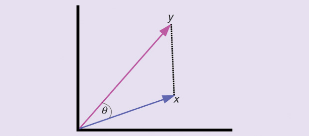
Various learning algorithms may implicitly or explicitly rely on a notion of distance (or similarity) between the objects of the data set. When using or customizing such algorithms for a particular application, the algorithm designer, or the practitioner, is usually faced with the following question: What could be a suitable faithful distance (or similarity) measure between the objects of the data set at hand? A faithful distance (or similarity) measure not only reveals the natural groupings and structure in the data, but it also improves the effectiveness and performance of any subsequent stages of data analysis, inference, prediction, or decision making (see Figure 1 and “Machine Learning: Basic Concepts and Terminology” for the difference between distance and similarity measures). In some settings, the data are already equipped with a notion of similarity or distance from the application domain, a priori knowledge, the physics of the problem, or the data-generating process. However, many times there are situations where such information on the data is not available, nor is it even possible to obtain. Thus, the designer and the practitioner have to face the tough question of how to define a faithful similarity or distance measure for the data set at hand.
[accordion title=”Machine Learning: Basic Concepts and Terminology”]
Distance versus similarity: These two terms carry common notions regarding how two different objects are distinct from or resemble each other. A distance function is a measure for the difference (or distinction) between two different objects from the same data set. The larger the distance, the more different the two objects are. A similarity function measures the resemblance between two different objects from the same data set. The larger the similarity, the more alike the two objects are. For instance, given two points in Cartesian coordinates, the distance between them can be measured using the Euclidean distance, while the similarity can be measured using the dot-product operation.
Supervised versus unsupervised learning: Two main learning settings exist in machine learning, supervised and unsupervised. In supervised learning, for each learning task, the data are given as pairs: the expected input and the expected (or desired) output for each object in the data set. The algorithm in this case has to learn the mapping from the expected input to the expected output. The role of the expected output is crucial; it guides or supervises the algorithm to learn the right mapping (as much as possible) for each input datum (and hence the name “supervised learning”). In unsupervised learning, for each learning task, the expected (or desired) output is not available. Hence, the algorithm has to learn a mapping and estimate the output without supervision. Obviously, unsupervised learning is more challenging than in the supervised setting. Typical examples for supervised learning problems are classification and regression problems, while clustering (partitioning the data into groups or hierarchies of similar objects) and density estimation (computing the probability of observing each given data point) are typical unsupervised learning problems.
Feature extraction: If the data set is not equipped a priori by its own distance or similarity measure, then a two-step approach is usually followed to define a distance (or similarity) measure between objects. First, each object is encoded into a set of numerical values that can best describe the sought characteristics of the objects; second, off-the-shelf distance (or similarity) functions are used in distance-based learning algorithms. The first step is known as feature extraction, which, itself, defines an enormous research discipline spanning various research topics [1]. Broadly speaking, feature extraction can be grouped into two categories: 1) engineered (and manually designed) feature extraction, which relies on a priori knowledge of the data, and 2) autonomous unsupervised feature learning, which makes minimal assumption on the data. Despite this dichotomy and the quantity of the literature, feature-extraction approaches ultimately encode each object into a vector, matrix, or tensor or into sequences of these structures when time is a characteristic of the data. The most common and notable representations, however, are vectors and matrices.
Dimensionality reduction: The task of dimensionality reduction is to reduce the number of variables of a given data set under consideration. It is a form of feature extraction, but it is more specific to high-dimensional vectors. There are two ways to achieve dimensionality reduction: variable selection/elimination and variable combination. The latter has also two variants: linear variable combination and nonlinear variable combination. Linear methods are exemplified by linear discriminant analysis and canonical correlation analysis, while nonlinear methods can be exemplified by manifold learning and spectral methods.
Kernel function: A kernel function measures the similarity between two input objects. It can be seen as a generalization for the dot-product operation in vector spaces. This function does so by computing the dot product between two input objects in some high- or even finite-dimensional feature space. Some examples include Gaussian kernels, polynomial kernels, exponential kernels, Laplace kernels, etc. Note that kernels do not actually map the objects into the high-dimensional feature space and then perform the dot-product operation to yield the final answer. Rather, they directly calculate the dot product without the need for mapping the data. This is known as the kernel trick.

Reference

1. I. Guyon and A. Elisseeff, “An introduction to variable and feature selection,” J. Mach. Learn. Res., vol. 3, pp. 1157–1182, Mar. 2003.

[/accordion]
The purpose of this article is twofold: first, to provide the reader with a brief overview of some well-known approaches for defining distances and similarity measures between data objects from the perspective of machine learning and pattern recognition; and second— and more importantly—to encourage the reader to consider a more fundamental, data-driven approach for defining distance and similarity between the objects of a data set. “Machine Learning: Basic Concepts and Terminology” provides explanations for some central ideas that will be discussed.

Off-the-Shelf Distance and Similarity Measures

If the data are in the form of vectors or matrices or have been transformed by feature extraction (see “Machine Learning: Basic Concepts and Terminology”) to such structures, then various off-the-shelf distance and similarity measures can be used. Some examples include Minkowski distances, the Mahalanobis distance, Matsushita distances, the chi-squared distance (for histograms), the Hamming distance, cosine similarity, dot products, kernels, angles between subspaces, and the Grassmann distance.
Using feature extraction and off-the-shelf distance functions has demonstrated reasonable success for various applications to date. However, as science is advancing and more types of complex data are being recorded, it is legitimate to ask whether such a rather naïve approach can be suitable for all types of data. A moment’s reflection should make it intuitively clear that any predefined distance function that is not adapted to the data under consideration cannot be expected to capture its intrinsic structure, regardless of any special-purpose feature extraction.
Hence, one can ask whether it is possible to design dataspecific and data-dependent distance functions that can capture some of the data’s intrinsic structure. Examples for such adaptive distance functions are dynamic programming-based distances such as the dynamic time warping (DTW) distance for time series and sequential data. Unlike the distance functions listed earlier, computing DTW requires defining three operations for any sequential data: insertion, deletion, and matching. Thus, DTW, by definition, is adapted for each data set through these operations. It is such an adaptation mechanism that we hope to adopt for defining data-dependent distance/ similarity functions.

Task-Specific Distance and Similarity Functions

I will first present two approaches that have already made significant improvements over the previous simple approach: 1) improving feature extraction such that off-the-shelf distance and similarity measures can perform better, and 2) learning task-specific distance and similarity functions. A feature these two approaches share is that the learning task should be known in advance. In other words, the distance (or similarity) function is task- and data-dependent. Furthermore, these approaches are limited to supervised learning settings.
For unsupervised learning, these two approaches can be useful for some problems such as clustering and dimensionality reduction when there are quantitative performance measures on the learning task, as well as model selection approaches for algorithms that solve these problems. Note that most of these approaches are also limited to data that are in vector format. Besides these two approaches, I will discuss kernel methods and their extensions to manifold learning algorithms. The power of kernel methods stems from their modularity and flexibility because they can operate on data in any form or structure in supervised and unsupervised settings.

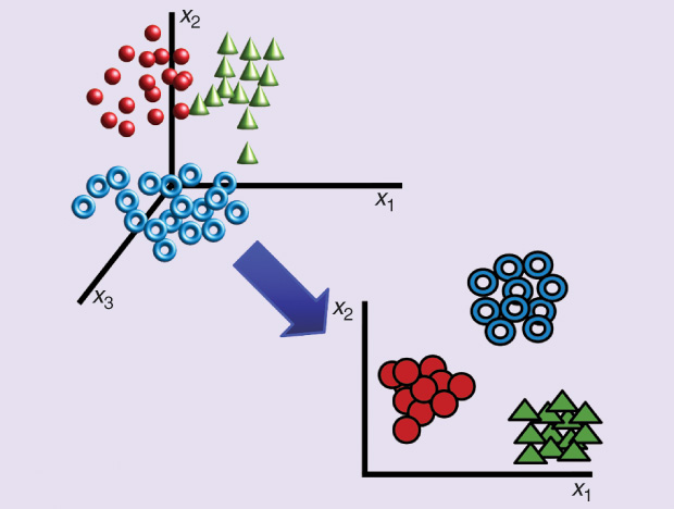
For approach 1), linear discriminant analysis (LDA) [2] (Figure 2) is one well-established technique. LDA learns a subspace that can, under some assumptions, best discriminate between two groups of observations: test case patients versus control patients, face images for person A versus person B, or spam versus nonspam e-mails, and the like. Projecting the data onto this subspace and applying a classifier based on the Euclidean distance or the Mahalanobis distance should yield the lowest possible classification error. Other approaches such as filters and wrappers have also shown to be effective.
For approach 2), distance metric learning (DML) algorithms are the only techniques available [3]. DML is very similar to LDA in its objective and its use, and it can be seen as the dual formulation of LDA. The novelty in DML, however, is that it directly addresses the problem of learning a distance function rather than learning a discriminative subspace, as LDA does. This different view yielded very modern and efficient algorithms for learning generalized quadratic distance functions.
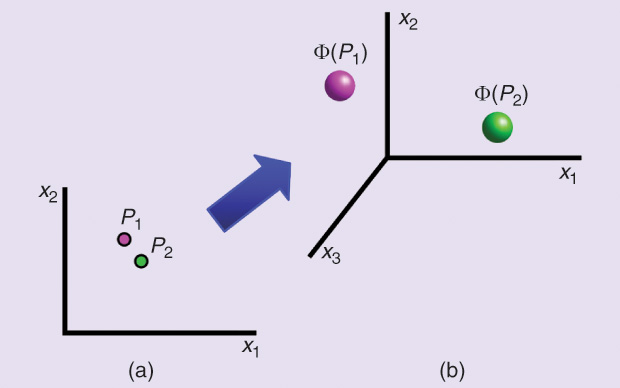
One approach that has had a great impact on machine learning is the introduction of kernel methods [4]. A main advantage of kernel methods is their modularity; they split the learning algorithm from the data. The learning algorithm operates on the data only through kernel operations between data objects in the feature space. The kernel function itself (Figure 3) does not need to be task-dependent, and, hence, it can be used in supervised and unsupervised learning algorithms. Note also that, in principle, for a specific learning task, a kernel-based algorithm can operate on any data as long as it is equipped with its proper kernel function. This, in turn, creates two challenges: 1) the need to design learning algorithms that can operate only on the data through kernels, and 2) the need to design proper kernels for every different type of data set; these are called data-dependent or data-specific kernel functions. Note that designing data specific kernels is very similar conceptually to the point I am making in this article. Note also that, usually, it is possible to obtain kernels from well-defined distance functions.

Manifold learning algorithms are special types of kernel methods. In particular, manifold learning algorithms are all based on the kernelized version of two classical linear dimensionality reduction algorithms from statistics and psychometrics: principal component analysis and classical multidimensional scaling. However, instead of using off-the-shelf kernels (radial basis function kernel, polynomial, etc.), they use data-dependent kernels. The differences among the various versions of manifold learning algorithms result from the different data-dependent kernel used by each algorithm. These algorithms were introduced in the unsupervised setting as nonlinear dimensionality reduction methods; that is, they learn a lower-dimensional Euclidean subspace where the data are nonlinearly projected onto it. Such a low-dimensional subspace represents a form of feature extraction as well. Assuming that the data-dependent kernel captures the data’s intrinsic structure, such low-dimensional Euclidean subspaces can be suitable for clustering and visualization because they tend to reveal the natural grouping and structure in the data. Again, the performance of such algorithms depends on faithful, data-dependent kernel functions.

Is There a Natural Distance Between Points in a Data Set?

The discussion here has so far presented the following approaches:

1. task-independent and predefined off-the-shelf distance (and similarity) measures
2. task-dependent feature extraction such that off-the-shelf distance functions perform better
3. direct learning of task-dependent distance metrics
4. kernel methods and manifold learning algorithms.

While all these approaches have shown success to date, the increasing data complexity raises the need for advanced approaches that can autonomously learn data-dependent distance (and similarity) functions, and capture the data’s intrinsic structure. These approaches should also be adaptive and flexible in order to transform them into task-dependent, supervised DML algorithms whenever needed.
To design such algorithms, the role of task-dependent feature extraction will continue to be crucial because it will allow us to handle complex objects such as Tweets, video clips, and fMRI data in clear, unified, well understood mathematical forms such as vectors and matrices. To begin a formal treatment, we assume that there is an abstract latent generating source for these vectors (or matrices). This source can be in the form of probability distributions or some dynamical system. If this source can be recovered in a formal manner, then the distance between outputs of this source can be fully recovered in a closed form, and such a distance can be considered the natural distance between objects. Alas, this is not the case! For instance, what is the formal model for the generating process of Tweets related to a topic on Twitter, or what is the formal model for the generating process of user ratings for a movie on Netflix [5]. While such a source likely exists, we also believe that recovering or identifying this source in a formal sense is very hard, if not impossible.

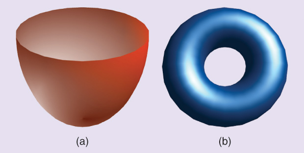
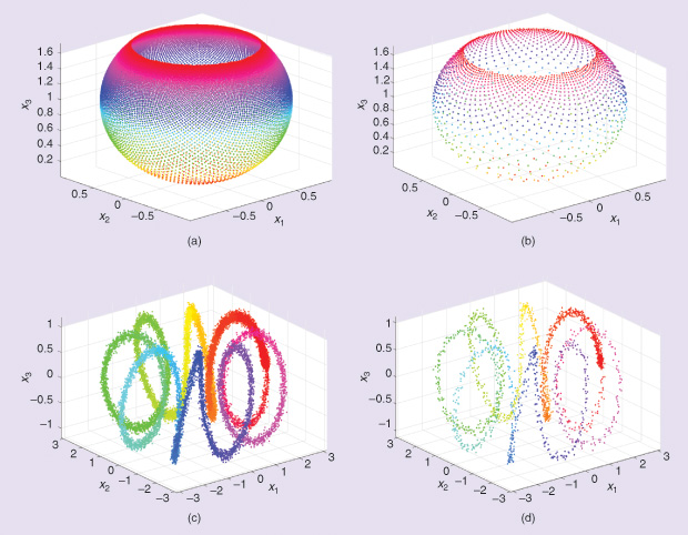
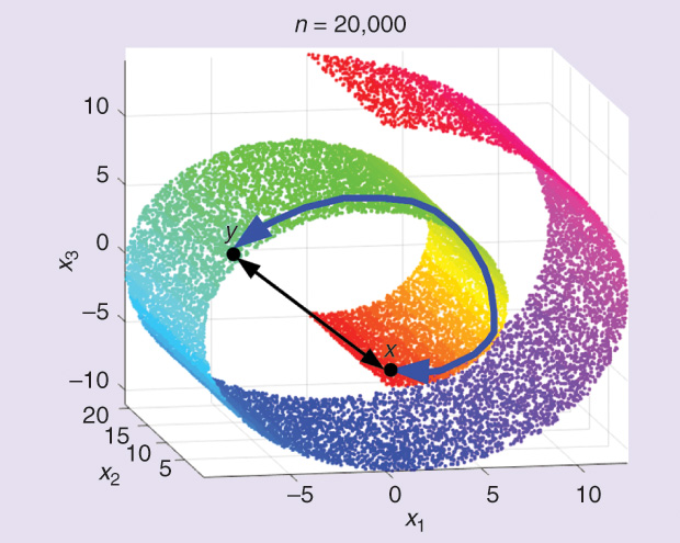
The situation, however, is not so daunting. Given an infinite amount of data from the unknown generating source, then such data will form what is known as the data manifold. To picture a manifold, consider lines and circles, which are one-dimensional manifolds (see Figures 4 and 5 for more complex examples). For complex nonlinear data, such manifolds are highly nonlinear and tangled. The distance between any two points on the data manifolds is simply the length of the shortest curve traversing the manifold between the two points. This known as the geodesic distance (Figure 6), and this is the natural distance for which we hope. The data set at hand, however, is finite, and it is usually considered a sparse, noisy sample from the data manifold. Hence, the best we can aim for is to approximate this natural distance using tools from linear algebra, statistics, probability, and theoretical computer science.

To some extent, the setting is similar to studying atoms in chemistry and physics. To the best of our knowledge, scientists did not actually see physical atoms. Rather, they observed the traces and signatures of atoms through different experiments. By studying these traces and signatures, they constructed accurate models for the atoms’ structure and properties that we know today. Similarly, we do not see the data generating process or the tangled nonlinear data manifold; however, through the sparse sample at hand, we can approximate the distance between points. The quality of the approximation depends on the samples’ density, as well as the complexity of the algorithms in terms of computing time and memory space. Note that, under this approach, approximating the natural distance is solely based on the data set at hand and is completely task-independent. Note also that this setup is aligned with the methodology of kernel methods that split the learning task from the similarity (or kernel) function.

An Interface Layer Between the Data and Learning Algorithms

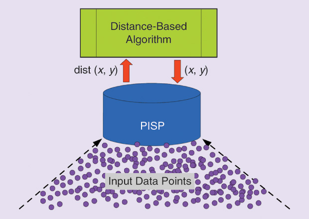
The setup and perspective introduced in the previous section encourage us to consider one approach for defining data-dependent distance functions. Current research work in this direction is one step toward approximating the geodesic distance from a finite data set [6]. This approach focuses on approximating the data manifold from the sparse data set at hand. This approximation is achieved by introducing an interface layer between the input data set and any distance-based algorithm (see Figure 7). If the algorithm queries the distance (or similarity) between two objects, then it sends this query to the interface layer, which approximates the data manifold. Thus, the distance provided by the interface layer is now a proxy for the distance between the objects of the given data set. For technical reasons, and due to its role, the interface layer is termed the pilot input space (PISP).
Figure 8 illustrates how the PISP approximates the data manifold through the “stitched” ellipsoidal patches. The PISP layer conveys to distance-based algorithms a new distance that considers intrinsic information in the data, such as the density of points and the approximate curvature (of the data’s underlying manifold). This interface layer provided systematic improvements for clustering algorithms and dimensionality reduction on various real data sets [6]. The chief result of the research on PISP presented here is that it confirmed the hypothesis that distances that consider intrinsic information, such as density and curvature, can increase the accuracy of distance-based data analysis and learning algorithms.

Some other works have proposed different types of distances to approximate the geodesic distance between points. For instance, in isometric embedding (isometric mapping) [7], the algorithm uses the elements (or objects) of the finite samples—say, vectors—as the vertices of a graph connecting the entire data set together. This is known as the data graph, or the neighborhood graph if each point is connected only to its few nearest neighbors. The distance between any two elements in the data set is taken as the length of the shortest path connecting these two elements on the data graph. In this setting, the data graph is assumed to approximate the manifold’s underlying topology, while the shortest path distance is assumed to approximate the geodesic distance. While the shortest-path distance is intuitively appealing, it is dependent and sensitive to the weights considered on the graph edges.
Density-based distances (DBD) and graph density-based distances [8] are other examples of distances that consider the data’s underlying density. Here, a distance between two points on a manifold is defined as the path connecting these two points such that paths passing through high-density regions should be much shorter than paths passing through low-density regions. Since there are possibly various paths connecting any two points, the DBD is defined as the shortest path connecting these two points. The intuition here is that, if the distance between a point and its few nearest neighbors is small, then it is expected that the neighborhood is a high-density region.
More fundamental approaches for distances that consider density information and curvature can be found in the literature on information geometry and computational information geometry. In this literature, divergence measures of information are the working horses for defining such distances. These measures quantify the discrepancy between probability distributions defined over an identical set of variables. Due to their technical involvement, these are not discussed in this article; interested readers are referred to [9] and [10].

Final Remarks

The ideas presented in the previous section define a new trend of distance measures different from the ones discussed earlier in the article. Such distance measures are learned in an unsupervised manner from the available finite samples and capture some of its intrinsic information such as density and curvature. The main advantage here is that the distance is data-dependent and not task-dependent, and hence, to a large extent, it can be used with any distance-based algorithm for analytics, data mining, or learning.
In addition, the mechanism for learning such distances can be transparently geared to be task-dependent, thereby fine-tuning the distance measure for specific tasks or types of analyses. The research in this area is relatively new and sparse among different research communities from different fields. This short overview is, indeed, neither complete nor comprehensive, and much more can be added. Nevertheless, the objective is to bring forward these ideas for readers and practitioners from different applied domains. I believe that the challenging demands from different application domains can thrust this research further ahead.

References

1. S. Shalev-Shwartz and S. Ben-David, Understanding Machine Learning: From Theory to Algorithms. New York: Cambridge Univ. Press, 2014.
2. R. A. Fisher, “The use of multiple measurements in taxonomic problems,” Ann Eugen., vol. 7, no. 2, pp. 179–188, Sept. 1936.
3. B. Kulis, “Metric learning: A survey,” Found. Trends Mach. Learn., vol. 5, no. 4, pp. 287–364, 2013.
4. B. Scholkopf and A. J. Smola, Learning with Kernels, Support Vector Machines, Regularization, Optimization, and Beyond. Cambridge, MA: MIT Press, 2001.
5. L. Valiant, Probably Approximately Correct. Nature’s Algorithms for Learning and Prospering in a Complex World. New York: Basic Books Inc., 2013.
6. K. T. Abou-Moustafa, D. Schuurmans, and F. P. Ferrie, “Learning a metric space for neighborhood topology estimation: Application to manifold learning,” J. Mach. Learn. Res. Workshops Conf. Proc., vol. 29, pp. 341–356, Nov. 2013.
7. J. Tenenbaum, V. de Silva, and J. Langford, “A global geometric framework for nonlinear dimensionality reduction,” Science, vol. 290, no. 5500, pp. 2319–2323, 2000.
8. S. Sajama, A. Orlitsky, “Estimating and computing density based distance metrics,” in Proc. 22nd Int. Conf. Machine Learning, 2005, pp. 760–767.
9. S.-I. Amari and H. Nagoka, “Methods of information geometry,” in Translations of Mathematical Monographs, vol. 191, American Mathematical Society. New York: Oxford Univ. Press, 2000.
10. F. Nielsen and R. Bhatia, Matrix Information Geometry. New York: Springer, 2013.