In the theory of relativity (TR), time dilation is a difference of elapsed time between two events as measured by observers either moving relative to each other or differently situated from gravitational fields [1], [2]. It means that astronauts return from space having aged less than those who remained on Earth; to the traveling party, those staying at home are living faster, while to those who stood still, their counterparts in motion lived at a slower rate. The theory predicts such behavior, and experiments have demonstrated it beyond doubt. The phenomenon is due to differences in velocity and in gravity (and it is called time dilation because the moving clock ticks slower). The effect would be greater if the astronauts were traveling nearer to the speed of light (approximately 300,000 km/s). Both factors—gravity and relative velocity—are the culprits and actually opposed one another.
Albert Eintein’s theory briefly states [3], [4]:
- In special relativity (hypothetically, far from all gravitational masses), clocks that are moving with respect to an inertial system of observation run slower. This effect is described by the Lorentz transformation.
- In general relativity, clocks within a gravitational field (as in closer proximity to a planet) are also found to run slower.
The first paper by Einstein, published in 1905, introduced the special relativity theory (SRT), and the second one, published in 1916, dealt with the much more difficult general relativity theory (GRT).
The Lorentz transformation (named for Hendrik Antoon Lorentz, 1853–1928) explains how the speed of light is independent of the reference frame. Lorentz shared the 1902 Nobel Prize in Physics with Pieter Zeeman (1865–1943) for the discovery and theoretical explanation of the Zeeman effect (the splitting of a spectral line into several components in the presence of a static magnetic field). The transformation describes how measurements of space and time by two observers are related, reflecting the fact that observers moving at different velocities may measure different distances and elapsed times. It was derived well before special relativity.
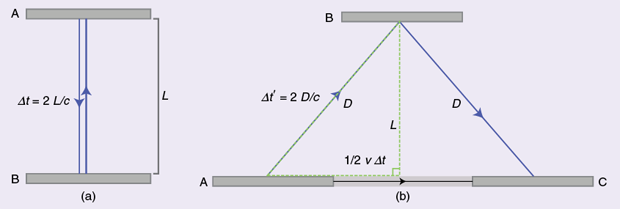
The first postulate of the TR, or principle of relativity, states that the laws of physics are the same in all inertial frames of reference. The speed of light c is constant in all reference frames, says the second postulate of the TR. Thus, the speeds of material objects and light are not additive. Consider a simple clock consisting of two mirrors, A and B, between which a light pulse is bouncing. The separation of the mirrors is L, and the clock ticks once each time the light pulse hits a given mirror. In the above figure (a), with a clock at rest, the light pulse traces out a path of length 2L, and the period of the clock is 2L divided by the speed of light
![]() (1)
(1)
From the frame of reference of a moving observer traveling at speed v [above figure (b)], the light pulse traces out a longer, angled path. Since the speed of light c is constant always and in all frames (second postulate), it implies a lengthening of the period of this clock from the moving observer’s perspective. That is, in a frame moving relative to the clock, the clock appears to be running more slowly. Application of the Pythagorean theorem leads to the well-known prediction of special relativity, i.e., the total time for the light pulse to trace its path is given by
![]() (2)
(2)
The length of the half path can be calculated as a function of known quantities as
![]() (3)
(3)
Substituting D from this equation into (2) and solving for Δt’ produces
 (4)
(4)
With the definition of Δt given in (1), the latter becomes
 (5)
(5)
In other words, for a moving observer, the period of the clock is longer than in the frame of the clock itself. It is a simple demonstration that only considers different speeds; if gravity is to be included, then things must be viewed by the more complex GRT.
A Few Scientific Events and Their Appearance in Time
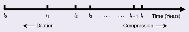
When taking a look at the scientific and technological historical evolution, one easily detects a time dilation if we explore the appearance of discoveries or inventions going backward, and a compression of time as we look forward, always from an arbitrary starting point. Intuitively, something like the graph shown above should be expected. Let us briefly review some specific examples: the measurement of blood pressure (BP), the development of the electrocardiograph, and that of computers.
The Measurement of BP
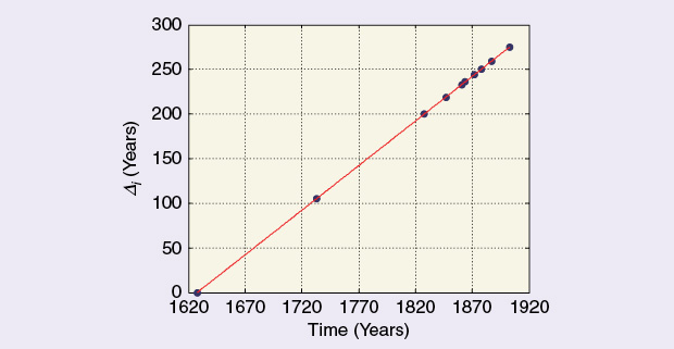
William Harvey (1578–1657) described the circulation of blood in 1628 but did not explain the force propelling the fluid around the body. In 1733, i.e., 105 years later, Stephen Hales (1677–1761) measured arterial pressure for the first time, while it took almost another century for the method to be improved by Jean Louis Marie Poiseuille in 1828 (1797–1869). Slowly, things began to speed up: Carl Ludwig (1816–1895) in 1847, Etienne Jules Marey (1830–1904) and Jean Baptiste Auguste Chauveau (1827–1917) in France in 1861, and Adolph Eugen Fick (1852–1937) in 1864 all introduced novel ideas applicable to the direct measurement of BP [5], [6]. From there on, knowledge and technological improvements increased fast, so much so that any attempt to organize them sequentially gets rather complicated as, sometimes, differences between one design and the next are quite small or not very significant. Ten points are depicted in the above figure, starting with William Harvey in 1628, even though he did not measure BP, but his work should be considered as a necessary predecessor. The abscissa represents the time in calendar years, while the vertical axis stands for the differences Δi with respect to the initial event. Table 1 summarizes the data for the ten points given in the figure. The compression effect is clearly seen.
Table 1 – Contributions to Arterial BP Measurement.
| Author | Year | Time Interval (Years) |
|---|---|---|
| Harvey | 1628 | 0 |
| Hales | 1733 | 105 |
| Poiseuille | 1828 | 200 |
| Ludwig | 1847 | 219 |
| Marey and Chauveau | 1861 | 233 |
| Fick | 1864 | 236 |
| Leonard Landois | 1872 | 244 |
| Golz and Gaule | 1878 | 250 |
| Rolleston | 1887 | 259 |
| Otto Frank | 1903 | 275 |
Data taken from Geddes’ textbook, 1970 [5]. Another source of information is the text by Paolo Salvi, 2012 [6].
Recording the Electrocardiogram
The development of the electrocardiogram (ECG) took approximately 50 years, without taking into account the contributions of the electronic and digital periods but with a preliminary period that started at the end of the 18th century and can be accepted as preparatory. The so-called Galvani’s Third Experiment demonstrated beyond doubt the existence of animal electricity. There were three communications by Galvani published in Latin in 1791 and 1792 as well as a third one, anonymously published by Galvani himself in Italian in 1793 [7]. Thus, the first date, 1791, could be taken as the initial point because it is when Galvani conceived the idea, even though his interpretation was wrong. Anyhow, differences of two or three years would not significantly influence the results.
The next step was made by Carlo Matteucci in 1842 [8], [9]. He had a frog gastrocnemius muscle stimulate the nerve of a second gastrocnemius and, in doing so, demonstrated the muscular electrical activity. Up to this moment, there were no actual records. Probably inspired by Matteucci, in 1856, Kölliker and Müller stimulated a sciatic nerve, which, in turn, triggered the contraction of its gastrocnemius mechanically linked to a kymograph (invented by Ludwig in 1846). That was a kind of crude ECG [10]. They did not publish these recordings. A Dutch researcher, F.C. Donders, repeated the experiment in 1872. We do not think the latter was a relevant contribution, though. Thereafter, and for about 10–15 years (1868–1883), the rheotome and the galvanometer became the recording technology—very laborious, indeed, but introducing digitalization (or sampling) as an essential concept long ahead of its time. Several ECGs were produced using this technique, all clustered within a few years (1877–1879). Interesting details are to be found in the textbook by Geddes and Baker [11]. In 1876, the first instrument that gave a continuous ECG was Lippman and Marey’s capillary electrometer, and the contemporaneous rheotome was quickly displaced. Based on the surface tension changes in mercury when traversed by a small electric current, it was really quite ingenious. Burdon-Sanderson and Page adopted the new instrument in 1878 and 1879. Waller, however, kept the electrometer a little longer, until 1887–1889, but his contributions should not be deemed significant within this context.
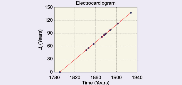
The last step was in the hands of Wilhelm Einthoven, who got manifestly tired of the capillary electrometer with all its inconveniences and errors and came up with his famous and much better string galvanometer in 1902–1903. His was a momentous apparatus, as relevant and significant for the development of electrocardiography as the kymograph was for BP recordings. Perhaps, the compression effect in this case is not very noticeable because of the rather short total time period (1842 or 1856–1903). Table 2 and the above figure were arranged using data from Geddes’ and Baker’s text [11].
Table 2 – Contributions to ECG Recording.
| Author | Year | Time Interval (Years) |
|---|---|---|
| Galvani | 1791 | 0 |
| Carlo Matteucci | 1842 | 51 |
| Ludwig | 1846 | 55 |
| Kölliker and Müller | 1856 | 65 |
| Donders | 1872 | 81 |
| Lippman and Marey | 1876 | 85 |
| Marchand | 1877 | 86 |
| Engleman | 1878 | 87 |
| Donders | 1879 | 88 |
| Page and Waller | 1880 | 89 |
| Waller | 1887 | 96 |
| Waller | 1889 | 98 |
| Einthoven | 1903 | 112 |
| Erlanger and Gasser | 1926 | 135 |
Development of Computers
Very early computer-related inventions, such as the abacus and calculators, are not accounted for here [12]. Apparently, the word computer was being used in 1613, and it applied to a person who performed calculations. At about the end of the 19th century, it began to be used to refer to a machine that performed calculations. In 1822, Charles Babbage (1791–1871) developed the difference engine, which was able to compute several sets of numbers. He was a British mathematician, philosopher, and mechanical engineer, also remembered for the concept of the programmable computer. Unfortunately, he was never able to complete the machine. Later, in 1837, Babbage proposed the analytical engine, with an arithmetic logic unit, basic flow control, and memory, but this computer was also never built. His youngest son, Henry Prevost (1824–1918), created six working difference engines based on his father’s designs, the last in 1910.
The Z1, built by Konrad Zuse in Germany in 1936–1938, was the first electromechanical binary programmable computer, really the first functional unit. Thereafter, the Colossus, recognized as the first electric programmable computer, was developed by Tommy Flowers in 1943. Between 1937 and 1942, John Vincent Atanasoff and Cliff Berry worked on what was the first digital computer (the ABC) at Iowa State University. It made use of vacuum tubes, binary arithmetic, and Boolean logic. [Thus, George Boole (1815–1864) should be included in this historic time line; he published his famous book, Laws of Thought, in 1854.] Of interest is that, in 1973, the U.S. Supreme Court declared that the Electronic Numerical Integrator and Computer (ENIAC), patented by J. Presper Eckert and John Mauchly, was invalid and named Atanasoff the inventor of the electronic digital computer. The ENIAC had been born during the period 1943–1946 at the University of Pennsylvania. Regretfully, only residual parts are now displayed in Philadelphia, after a rather painful history. In 1949, the British unit known as the Electronic Delay Storage Automatic Calculator (EDSAC) was launched, with thefirst stored program, while the Universal Automatic Computer I (UNIVAC I) was the second commercial computer produced in the United States, mainly designed by the already experienced Eckert and Mauchly. Konrad Zuse began working on the Z4, which became the first commercial computer in 1950. The 701 (the first mass-produced piece) was introduced in 1953 by International Business Machines (IBM). People in Japan were active in the field, too: a general-research group was formed at the University of Tokyo, led by Hideo Yamashita with the participation of Toshiba Company. After many problems as well as personnel turnover, a machine was completed in 1959, but operation was stopped in 1962. It was named TAC. The first computer with random access memory was the WHIRLWIND, developed in 1955 at the Massachusetts Institute of Technology (MIT), and the Transistorized Experimental Computer (TX-O) was demonstrated at MIT in 1956. Thereafter, in 1958, Nippon Electric Company finished the NEAC-1101, using the parametrons invented by Eiichi Goto (1931–2005) in 1954. In 1960, Digital Equipment Corporation released its first of many programmed data processor (PDP) computers, the PDP-1, a rather small unit. (Coauthor Max E. Valentenuzzi used a PDP-8S in 1968 to process numerical data for his Ph.D. dissertation.) Hewlett Packard released a general computer, the HP-2115, in 1966 and began marketing the first mass-produced PC, the HP 9100A, in 1968. The first portable computer, the IBM 5100, was released in 1975. Steve Wozniak designed the first Apple I in 1976, and IBM came up with the first personal computer, called the IBM PC, in 1981.
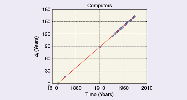
Thereafter, the flood of inventions and new developments seemed like an endless waterfall, and it is still flowing today. Table 3 and the figure above briefly summarize these data. In fact, it becomes increasingly difficult to separate out relevant from less-relevant contributions.
Table 3 – The Development of computers
| Author/Development | Year | Time Interval (Years) |
|---|---|---|
| Charles Babbage | 1822 | 0 |
| Charles Babbage | 1837 | 15 |
| Henry Babbage | 1910 | 88 |
| Z1—Konrad Zuse | 1938 | 116 |
| ABC | 1942 | 120 |
| Colossus—Tommy Flowers | 1943 | 121 |
| ENIAC | 1946 | 124 |
| EDSAC | 1949 | 127 |
| UNIVAC I | 1949 | 127 |
| First Commercial Computer: Z4R by K. Zuse | 1950 | 128 |
| IBM 701 and MIT WHIRLWIND | 1953 | 131 |
| MIT WHIRLWIND | 1955 | 133 |
| TX-O | 1956 | 134 |
| NEAC 1101 | 1958 | 136 |
| Toshiba | 1959 | 137 |
| PDP-1 | 1960 | 138 |
| PDP-8/S | 1965 | 143 |
| HP-2115 | 1966 | 144 |
| HP 9100A | 1968 | 146 |
| INTEL 4004 | 1971 | 149 |
| XEROX ALTO | 1974 | 152 |
| ALTAIR | 1975 | 153 |
| IBM 5100 | 1975 | 153 |
| Apple I | 1976 | 154 |
| IBM PC | 1981 | 159 |
| OSBORNE I | 1981 | 159 |
| COMPAQ PC-CLONE | 1983 | 161 |
| IBM Portable | 1984 | 162 |
| IBM-PCD | 1986 | 164 |
Discussion
From the very beginnings of man up to now, an acceleration of discoveries and inventions has taken place: from fire to wheel; from herbal medicine to more sophisticated drugs; and from mechanical technologies to more elaborate chemical, electromechanical, and electronic methods. Thus, the time interval between discoveries and inventions gets longer when going back in the history of science and technology, i.e., there is a dilation of time. It becomes shorter as we explore the development of knowledge coming toward the present, i.e., a time-compression effect occurs (Figure 2).
One obstacle that often comes up is the determination of how important, relevant, or significant a given contribution is. When facing breakthroughs like Ludwig’s kymograph, Mendeleiev’s table, Einstein’s relativity, or the discovery of DNA, not even the shadow of a doubt hinders their inclusion as highly significant scientific events. The question becomes diffuse in the case of those secondary contributions that somewhat improved the contemporary knowledge of a certain subject area.
One may pose an epistemological question: is there a limit to such compression? In fact, it is a knowledge phenomenon. Knowledge feeds itself as one discovery stands on the shoulders of previous ones. Well, actually, there is nothing new in repeating this concept (nihil novum sub solem). A second question seems more daring: Is there a law that might predict the next interval? The absurd would perhaps lead us to think that a continuum of newer and newer products could take place. And such an idea brings up the concept of the mind’s infinite creative power, obviously helped by technology. Would it be conceivable to adapt (or fit) and apply Einstein’s equation? Admittedly, it sounds preposterous, for what would take the place of the speed of light? A recent article by Arbesman [13] tries to somehow quantify the ease of scientific discovery, and, in several respects, it brings about more questions than answers, but it sounds like a well-thought attempt.
Another aspect to recall refers to psychological time, i.e., the perception of time according to different circumstances: time in childhood (one year looks very long), time in old age (one year feels short), time during sickness (a few days in a hospital are endless for a patient in pain), time as a student during an exam (an hour is all morning), time of pleasure is short, time for an inmate in prison is exceedingly long. Coauthor Max E. Valentinuzzi’s father, also named Max Valentinuzzi (1907–1985) said, back in 1934 that time is inseparable from the patient, that time is part of clinical phenomena [14]. Borges (1899–1986), in a short philosophical essay [15], stated that the present is as evasive as the concept of geometrical point (as on a line, a plane, or in space); in fact, the present point does not exist, because it is past and it is also future, and thus, it touches both.
We think the three examples reviewed here acceptably show the time-compression effect in discoveries and inventions. Other subject areas, such as genetics, telecommunications, cars, or aviation, should be studied by epistemologists to better visualize the phenomenon.
References
- (2013, Mar. 19). [Online]. Available: http://en.wikipedia.org/wiki/Time_dilation
- J. L. A. Francey, Relativity. Australia: Longman, 1974.
- A. Einstein, “Zur Elektrodynamik bewegter Körper [In German, On the electrodynamics of moving bodies],” Annalen der Physik, vol. 17, ser. 4, pp. 891–921, 1905.
- A. Einstein, “Die Grundlage der allgemeine Relativitätstheorie [In German, The foundations of the General Theory of Relativity],” Annalen der Physik, vol. 49, no. 7, pp. 769–822, 1916.
- L. A. Geddes, The Direct and Indirect Measurement of Blood Pressure. Chicago, Il: Year Book Medical Pub., 1970.
- P. Salvi, Pulse Waves: How Vascular Hemodaynamics Affects Blood Pressure. Milan, Italy: Springer-Verlag, 2012.
- H. E. Hoff, “Galvani and the pre-Galvani electrophysiologists,” Ann. Sci., vol. 1, pp. 157–172, 1936.
- C. Matteucci, “Correspondence,” Comptes Rendus de l’Academie des Sciences de Paris, vol. 159 (Suppl. 2), pp. 797–798, 1842.
- C. Matteucci, “Sur un phénomène physiologique produit par les muscles en contraction,” Annales de Chimie et Physique, vol. 6 (Suppl. 3), pp. 339–343, 1842.
- R. A. Kölliker and J. Müller, “Nachweiss der negativen Schwankung des Muskelstroms am natürlich sich contrahirenden Muskel [In German, Proof of the negative deviation given by the muscular current during the natural muscle contraction],” Verhandlungen der Physikalisch-Medizinischen Gesellschaft zu Würzburg, vol. 6, pp. 528–533, 1856.
- L. A. Geddes and L. E. Baker, Principles of Applied Biomedical Instrumentation, 2nd ed. New York: Wiley, 1975.
- Computer Hope. (2013). Available: http://www.computerhope.com/issues/ch000984.htm.
- S. Arbesman. (2012). Quantifying the ease of scientific discovery. Scientometrics [Online]. 86(2), pp. 245–250.
- M. Valentinuzzi, “El tiempo en los fenómenos clínicos [In Spanish, Time in clinical phenomena],” Actualidad Médica Mundial, vol. 4, no. 47, pp. 401–404, Nov. 1934.
- J. L. Borges, “Borges oral: El tiempo,” in Obras Completas. Buenos Aires: Editorial Sudamericana, June 23, 2011, pp. 206–214.