Intracardiac Pressure–Volume Diagrams and Their Links with Thermodynamics

Work and energy, power and efficiency, all four involve concepts that seemingly belong only to machines… but much before they popped out of fire and coal, live beings possessed and used them as essential life-supporting intrinsic attributes.
The main objective of this column is to historically connect the pressure–volume diagram (PVD) of the heat mechanical engines and that of the heart—a natural chemical engine—both types being generators of useful work.

Beginning with Some Thermodynamics

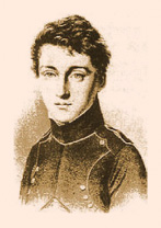In 1824, Nicolas Léonard Sadi Carnot (1796–1832) (right) published in Paris a little book Réflexions sur la Puissance Motrice du Feu et sur les Machines Propres a Développer cette Puissance (Reflections on the Motive Power of Fire and on the Machines Adequate to Develop Such Power), written in one shot, with no chapters, sections, or subtitles, some mathematics, and only a few simple figures and tables. Many years later, in 1872, the Annales de l’École Normale Supérieure (2^e série, tome 1, pp. 393–457) republished the book, also in Paris, and later on, in 1897, an English translation was produced by R.H. Thurston, with comments by Lord Kelvin (William Thomson, 1824–1907), including other related material to expand the subject. The latter two versions can be located on the Internet [1], [2]. A few original copies can still be found in some bookstores, a jewel for any library, indeed. There is also a Spanish translation by J. Cabrera, who used to be a professor in Zaragoza, published in 1927 in Madrid, Spain.
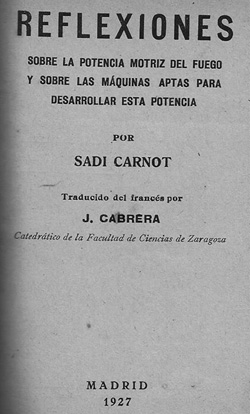Right: The front page of the Spanish translation of Nicolas Léonard Sadi Carnot’s only book. This edition has an extension of 127 pages. (Image courtesy of Max E. Valentinuzzi.)
Carnot was a military engineer and physicist, now recognized as the father of thermodynamics because of the concepts introduced in his only publication, where he gave the first successful theory of the maximum efficiency of heat engines. Unfortunately, he retired from the army at a young age in 1828, without a pension, and had to be interned in an asylum in 1832 as suffering from “general delirium,” whatever that term meant in those days; Carnot died of cholera shortly thereafter at age 36.
The principle enunciated by Carnot constitutes the second law of thermodynamics, i.e., it is impossible to extract an amount of heat from a hot reservoir and use it all to do work, as some amount of heat must be exhausted to a cold reservoir. This fact precludes a perfect heat engine. He introduced with it the concept of a heat engine’s ideal cycle. It can be shown that it is the most efficient cycle for converting a given amount of thermal energy into work or, conversely, creating a temperature difference (refrigeration) by doing a given amount of work. The ideal or perfect Carnot engine is only a theoretical limit and cannot be built in practice. The Carnot cycle consists of four stages:
1) Isothermal expansion at a high temperature T1 (point A to point B, figures below). The gas expands, doing work on the surroundings without changing its temperature. There is absorption of heat Q1 and of entropy S from the high temperature reservoir.

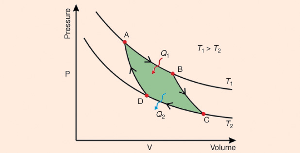
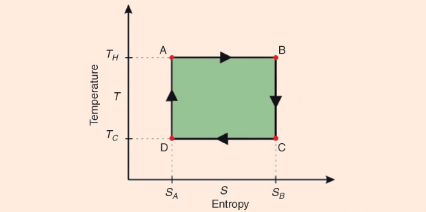
2) Isoentropic expansion of the gas (point B to point C, figures above). The engine is assumed to be thermally insulated so that it neither gains nor loses heat, i.e., it is an adiabatic process. The gas continues to expand performing work on the surroundings, while losing an equivalent amount of internal energy. Such expansion causes it to cool to temperature The entropy remains unchanged. Remember that entropy, is a measure of disorder or a measure of decay toward thermodynamic equilibrium, which in isolated systems corresponds to the maximum entropic state.
3) Isothermal compression of the gas at a low temperature T2 (point C to point D, Figures 3 and 4). The surroundings do work on the gas, causing an amount of heat energy Q2 and entropic change ΔS = Q2/T2 to flow out of the gas to the low temperature reservoir, which is the same amount of entropy absorbed in step 1.
4) Isoentropic compression of the gas (point D to point A, Figures 3 and 4). Once again, the mechanisms of the engine are assumed to be thermally insulated, again adiabatic. During this step, the surroundings do work on the gas, increasing its internal energy and compressing it, causing the temperature to rise to The entropy remains unchanged. The gas has returned to the starting point A.
The amount of energy transferred as work is

The efficiency η is defined as W/Q1 where W stands for the work done by the system (energy exiting as work) and Q1 represents the heat getting into the system. The temperature is always given in absolute terms, that is, [°K] = [°C] + 273.15, a reminder of the well-known Celsius–­Kelvin relationship. The Carnot cycle is totally reversible, so becoming a refrigeration cycle. It remains the same except that the directions of any heat and work interactions move in opposite directions if compared to the previous case. In addition, we should recall that temperature is a number related to energy, but it is not energy itself. It relates to the average kinetic energy of the molecules of a substance.
Carnot’s work attracted little attention during his lifetime, but it was later used by another French engineer, Émile Clapeyron (1799–1864), the German physicist and mathematician Rudolf Clausius (1822–1888), and Lord Kelvin (mentioned earlier, born the year Carnot published his seminal book) to further develop the field of thermodynamics. For the sake of completeness, let us remember, in simple terms, that the first law of thermodynamics is a version of the law of conservation of energy, which states that the total energy of an isolated system is constant: energy can be transformed from one form to another but cannot be created or destroyed. The third law of thermodynamics states that the entropy, defined as S = Q/T (heat quantity divided by absolute temperature), contained by any pure substance in thermodynamic equilibrium approaches zero as the temperature approaches zero. The entropy of a system at absolute zero is zero.

Early heat Engines

Fire is obviously not an engine, but it is a combustion process of some substance source of energy that, in the end, allowed and led to the invention and development of the heat engines. Its discovery and control was one of the earliest of human findings. Its origins can be traced back to the Early Stone Age (Lower Paleolithic), perhaps at a site named Gesher Benot Ya’aqov, in Israel, where charred wood and seeds were recovered and dated around 790,000 years old [3]. The subject is quite interesting and with abundant literature [4], [5]. Materials to produce fire from wood, coal, petroleum, or others belong to a different chapter of history and technology. In fact, what is desired is heat, expressed in calories, and the more per unit of the source that is combustible, the better for the user as efficiency improves. Centuries went by before an actual thermal engine was built, deriving its power output from the good old fire. Carnot was well aware of the subject and mentioned several names that put effort in its development, all settled in England, as he clearly said in his book. They are somewhat entangled and with several smaller inventions and pieces of knowledge that, in a relatively short period, produced the steam engine and, with it, triggered the Industrial Revolution (from ~1760 to ~1840), which has been well studied and discussed by historians.
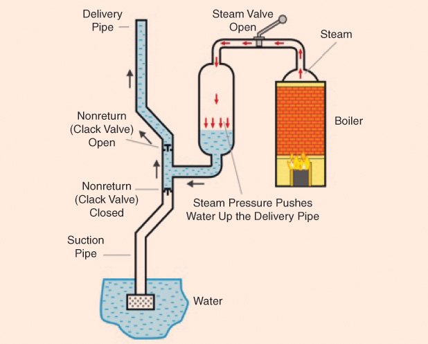
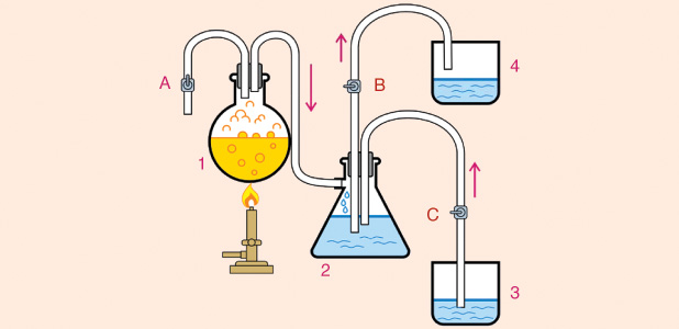
Thomas Savery (1650–1715) was born at Shilstone, a manor house near Modbury, Devon, England. He invented the first steam-powered engine, filing a patent in July 1698 that later led to the Fire Engine Act issued by the British Parliament. The patent covered all engines that raised water by fire. Savery’s engine had no piston and no moving parts except for the taps. It was operated by first raising steam in the boiler, from where it was then admitted to a vessel. As the steam pressure built up, it produced a suction effect that took water from the bottom of the mine; this action was the main purpose of the machine (Figures below). This machine, even though it worked, was plagued with several problems.

Fourteen years later, in 1712, Thomas Newcomen (1664–1729), an ironmonger who also worked with Savery, came up with his atmospheric engine, which was the first practical device to generate mechanical power from steam more efficiently. Interest in these machines was growing quickly, and several mechanical engineers tested new ideas. Scottish engineer James Watt (1736–1819) designed an improved version of the Newcomen engine. As a result, Watt is today better known than Newcomen in relation to the origin of the steam engine. Watt realized that the early engines wasted a great deal of energy by repeatedly cooling and reheating the cylinder, so he introduced important details, such as a separate condenser, making steam engines more cost-effective. He developed the concept of horsepower, taking the power produced by a horse at work as a reference since horses were the main natural “machines” people had at hand. Watt was elected a Fellow of the Royal Society of London in 1785.

Another contributor to steam engine development was John Smeaton (1724–1792), a civil engineer and eminent physicist. Smeaton experimented with Newcomen’s machine and made significant improvements around the time James Watt was building his first engines (late 1770s). Smeaton’s interests were certainly wide-ranging, and he was always aware of what his contemporaries were doing. He collected data from 15 working engines in the Newcastle area and 12 in Cornwall, expressing the results in terms of their power and efficiency. He built an experimental engine in 1770 and began rigorous testing. After two years’ work, he drew up a comprehensive table of data. He designed 13 engines altogether, four of them with waterwheels. In 1783, he produced a machine that was able to raise 13.3 t of coal per hour from a depth of 174 m, which was quite an accomplishment. It was to be his last steam engine [6]. Smeaton enjoyed a long series of correspondence with Watt and his associate Matthew Boulton (1728–1809).
Still, there are two more who were engaged in the steam engine saga, also mentioned by Carnot: Arthur Woolf (1766–1837) and Richard Trevithick (1771–1833). Woolf was famous for inventing a high-pressure compound steam engine. Trevithick invented a high-pressure steam engine and the first railway steam locomotive, which, on 21 February 1804, hauled a train along the tramway of the Penydarren Ironworks in Wales. Trevithick also worked as a mining consultant in Peru. At one point, he faced financial ruin, also suffering the strong rivalry of other engineers, and, near the end of his life, he fell out of the public eye.

PVDs

All of these heat engines (or thermal engines) can be characterized by their PVDs, or pressure–volume loops (PVLs), and they constitute a whole chapter in current courses of thermodynamics, eventually becoming a headache for students. A PVD describes the cyclic changes in the volume and pressure in a system. On an oscilloscope screen, when adequately inputting the component signals, respectively—on the horizontal and vertical axes after turning off the scanning circuit—they are akin to the traditional Lissajous figures (named after Jules Antoine Lissajous, 1822–1880). However, PVDs now are not the exclusive property of mechanical engineers, for they are also useful in cardiovascular and respiratory physiology. Originally called indicator diagrams, they were developed in the 18th century, long before Carnot introduced his ideal cycle, as tools for understanding and evaluating the efficiency of steam engines. An ideal PVD looks like the one shown in Figure 4, except that the horizontal axis represents volume and the vertical axis stands for pressure. A key feature of the diagram is that the amount of energy expended or received by the system as work can be estimated as the area under the curve on the chart. For a cyclic diagram, the network is that enclosed by the curve. In a real device, the loop shape is curved, although the four phases are easily detected.
The PVD was actually developed by Watt and his employee John Southern (1758–1815) to estimate the engine’s efficiency. In 1796, Southern devised a simple technique to generate the diagram by fixing a board while the piston traced the “volume” axis through a lever gadget; simultaneously, a pencil attached to a pressure gauge moved at right angles to the piston drew “pressure” (we do not know what kind of pressure gauge he used). Thus, Watt could calculate the work done by the system. However, other people had similar ideas, and some litigation took place over patent ownership. The actual fact is that Watt used the diagram to make radical improvements to the steam engine and kept it a trade secret. However, it was made public in an anonymous letter in 1822 [7]. Later, in 1834, Clapeyron used the PVD to better explain the Carnot cycle, bringing it to a central position in thermodynamics [8].

Intraventricular PVDs

Until this point, everyone referred to engineering, mostly mechanical, as well as applied physics when dealing with heat and energy. The last date we have listed is 1834, when physiologists were still struggling with the measurement of blood pressure. Karl Ludwig’s kymograph was introduced over a decade later, in 1847 [9]. Volume, in turn, appeared as a rather obscure cardiovascular variable. The question arises as to when, who, and how the PV concept got into physiology; it is a concept that is in the realm of bioengineering, for it is true physics knowledge applied to biology.
Apparently, more than 50 years elapsed before the first PVD description of a heart was written by the German physiologist Otto Frank, in 1899 [10], using experimental data previously observed in frog ventricles [11]. He studied medicine in München and Kiel with later courses in mathematics, chemistry, physics, anatomy, and zoology in other universities. In addition, Frank worked until 1894 as an assistant to Carl Ludwig in Leipzig, where he completed his doctoral degree. Thus, he was a well-trained scientist aware of the then-current advances. It is very likely that Frank was also updated regarding thermal engines and probably saw similarities with the heart; it must have been easy for him to extend the PVD concept to that organ, which is considered to be a chemical machine.
In 1914, Patterson and his group redrew Frank’s diagram, trying to interpret it in terms of length and tension. They even extrapolated these results to a canine heart weighing approximately 70 g [12]. However, the detection of volume always remained a variable not amenable to straightforward transduction. In more recent times, echocardiography was used extensively in different ways to estimate volume. X-rays and radionuclide ventriculography have also been applied in several modalities. Single photon emission tomography was another not very successful proposal. Regretfully, all of these methods are based on simple geometrical models of the heart cavities, require elaborate computations, or call for expensive equipment, and the error margins are always substantial [13]. Besides, the loops required a more stringent methodology and interpretation when dealing with cardiac function; for in the end, they are a magnificent quantitative tool to evaluate how well the heart operates.
The problem of detecting volume found a possible first answer by the application of the impedance technique in 1966 by a group led by Leslie A. Geddes, in Houston, Texas [14], [15]. Thereafter, and starting in the late 1970s, a Dutch team under the direction of Jan Baan introduced independently the conductance catheter as a more elaborate development, publishing a number of important papers of which, perhaps the most relevant, is one that appeared in 1984 [16]. The interpretation and methodology were well tackled by Kiichi Sagawa’s group at Johns Hopkins University, from where a long series of papers was summarized in an outstanding book in 1988 [17]. Quite independently, another group in South America developed a system that led to several papers of which the three first were published in 1986 [18]–[20]. The figure below shows an early result obtained by the Tucumán, Argentina, group. Thereafter, and for some time, the three groups got in touch and exchanged information.

The field has advanced enormously since the 1990s, with improvements in the conductance catheter and applications in transgenic rats and mice [21]. Other more recent publications delve into more specific aspects of ventricular thermodynamics [22]. However, we will not continue referencing other papers because this is not a review column.

Discussion

We have concentrated on the intracardiac PVD, giving examples obtained from the left ventricular cavity; however, the other chambers are perfectly amenable for similar studies. The right ventricle, however, has a peculiar shape that tends to make the procedure somewhat more difficult and has been less studied than the left side. In 1988, for example, Redington and collaborators analyzed the normal right ventricular PV relationship by recording biplane ventriculograms with simultaneous high-fidelity pressure recordings in ten adults. The right ventricular volume was measured frame by frame from digitized ventriculograms by a modification of the well-known Simpson’s rule (credited to the mathematician Thomas Simpson, 1710–1761, of Leicestershire, England). The accuracy of this method was tested in a study of 22 human and animal right ventricular casts. The derived regression equations were used to correct the right ventricular volumes calculated from in vivo studies. The mean ± SD end diastolic volume index for the group was 62 ± 13 ml/m², the stroke volume index was 43 ± 8 ml/m², and the ejection fraction was 62 ± 6%. The normal right ventricular PVD was triangular, departing significantly from the more typical squarelike shape of the normal left PVD. Ejection from the right ventricle began early during the pressure rise and continued as the right ventricular pressure fell. As a result, phases of isovolumic contraction and relaxation were difficult to define. These observations show that the normal right ventricular PVD differs considerably from those of the normal left ventricle, presumably reflecting the different loading conditions of the two ventricles [23].
The two atria are also possible targets to be functionally evaluated by the PVD, unfortunately with far fewer reports than the ventricles. It must be noted that the left atrium, particularly due to its anatomical position, cannot be reached by catheterization and requires direct puncturing of its wall. Ferguson and collaborators from Boston, Massachusetts, recognized in 1989 that the assessment of the relationship between pressure and volume in the right atrium had been hampered by difficulties in the measurement of atrial volume. They detected the latter with an impedance catheter, being able to study right atrial PVDs in patients without atrial septal defect, which exhibited the normal figure eight pattern, that is, showing an A-loop (atria contraction) and a V-loop (passive filling), corresponding to the A- and V- of right atrial pressure, respectively. During inspiration, the mean right atrial pressure decreased and the mean right atrial volume increased, consistent with augmented venous return. With the Valsalva maneuver, the right atrial pressure increased and both the right atrial stroke volume and mean right atrial volume decreased compared with baseline. Ferguson et al. concluded that the impedance catheter provided a useful method of assessing dynamic changes in the human right atrial PV relationship [24].
Regarding the left atrium, we could only locate a report by Kasses and Kennedy, in 1969 [25], where the left atrial volume and pressure measurements in 23 normal subjects and 117 cardiac patients were compared with several electrocardiographic criteria for left atrial disease; however, no PVLs were obtained. It is hard to believe that no one has ever at least tried to record the left atrial diagram in an animal experiment. More common are the attempts to correlate pressure and volume estimations in echography studies, with no aim to measure the atrial pump efficiency but to obtain indirect pressure or volume measurements in the atria [26].
Finally, since the PVD also finds a place in the study of the respiratory system, although the latter was not within the purposes of this article, we should mention the review by Qin Lu and Louby, from the University of Paris VI, France [27].

Conclusions

The origins of the PVD concept of thermal engines have been acceptably presented. To find out exactly how James Watt implemented the diagram recording would require digging into the original patents, a good project for a professional young historian. There seems to be a gap between Carnot’s book (1824) and Otto Frank’s first cardiac loop (1899), with Carl Ludwig’s clear and also practical physics–mathematical concepts looking into the physiological sciences (1847) as a bridge joining both. The application of the PVD to respiratory physiology now appears to be a natural consequence; however, it remains to be determined when the concept was first applied to that area. This column did not try to explore the latter. Visit Mashpedia to see numerous PVDs shown in videos.

Acknowledgments

We would like to thank Gustavo Idemi, a professional artist from the city of San Juan, West Argentina (just by the Andean chain), who kindly redrew and modified Figures 3–6 in this article.

References

1. S. Carnot. (1872). Réflexions sur la puissance motrice du feu et sur les machines propres a développer cette puissance, Ann l’École Normale Supérieure, 2esérie, tome 1, pp. 393–457. [Online].
2. N. L. S. Carnot. (1897). Reflections on the Motive Power of Heat. [Online]. London: Chapman & Hall.
3. N. Goren-Inbar, N. Alperson, M. E. Kislev, O. Simchoni, Y. Melamed, A. Ben-Nun, and E. Werker, “Evidence of hominin control of fire at Gesher Benot Ya`aqov, Israel,” Science, vol. 304, no. 5671, pp. 725–727, Apr. 2004.
4. K. Kris Hirst. (2014). The discovery of fire and human-controlled fire use. About.com Archaeology. [Online].
5. M. J. Church, C. Peters, and C. M. Batt, “Sourcing fire ash on archaeological sites in the Western and Northern Isles of Scotland. Using mineral magnetism,” Geoarchaeology, vol. 22, no. 7, pp. 747–774, 2007.
6. (2014). About John Smeaton, Engineering Timelines. [Online]. The Web site offers also a list of references.
7. Anonymous, “Account of a steam-engine indicator,” Quart. J. Sci., vol. 13, p. 95, 1822.
8. E. Clapeyron, “Mémoiresur la puissance motrice de la chaleur (Memoir on the motive power of heat),” J. de l’École Royale Polytechnique, vol. 14, no. 23, pp. 153–190, 1834.
9. M. E. Valentinuzzi, K. Beneke, and G. E. González, “Ludwig: The bioengineer,” IEEE Pulse, vol. 3, no. 4, pp. 68–78, 2012.
10. O. Frank, Die Grundform des arteriellen Pulses [Basic shape of the arterial pulse], Zeitschriftfür Biologie, vol. 37, pp. 483–526, 1899. (A translation is given by K. ­Sagawa, R. K. Lie, and J. Schaefer, J. Mol. Cell Cardiol., vol. 22, pp. 253–277, 1990).
11. O. Frank, “ZurDynamik des Herzmuskels [On the cardiac muscle dynamics],” Zeitschrift für Biologie, vol. 32, pp. 370–437, 1895.
12. S. W. Patterson, H. Pipper, and E. H. Starling, “The regulation of the heart beat,” J. Physiol. (London), vol. 48, pp. 465–513, 1914.
13. M. E. Valentinuzzi and J. C. Spinelli, “Intracardiac measurements with the impedance technique,” IEEE Eng. Med. Biol. Mag., vol. 8, no. 1, pp. 27–34, 1989.
14. L. A. Geddes, H. E. Hoff, and A. Mello, “The development and calibration of a method for the continuous measurement of stroke volume in the experimental animal,” Jpn. Heart J., vol. 7, pp. 556–565, 1966.
15. L. A. Geddes, H. E. Hoff, A. Mello, and C. Palmer, “Continuous measurement of ventricular stroke volume by electrical impedance,” Cardiovasc. Res. Ctr. Bull., vol. 4, no. 4, pp. 118–130, 1966.
16. J. Baan, E. T. van der Velde, H. G. de Bruin, G. J. Smeenk, J. Koops, A. D. van Dijk, D. Temmerman, J. Senden, and B. Buis, “Continuous measurement of left ventricular volume in animals and ­humans by conductance catheter,” Circulation, vol. 70, no. 5, pp. 812–823, 1984.
17. K. Sagawa, L. Maughan, H. Suga, and K. Sunagawa, Cardiac Contraction and the Pressure-Volume Relationship. New York: Oxford Univ. Press, 1988.
18. O. E. Clavin, J. C. Spinelli, H. Alonso, P. ­Solarz, M. E. Valentinuzzi, and R. H. Pichel, “Left intraventricular pressure-­impedance diagrams (DPZ) to assess cardiac function. Part I: Morphology and potential sources of artifacts,” Med. Prog. Technol., vol. 11, pp. 17–24, 1986.
19. J. C. Spinelli, O. E. Clavin, E. I. Cabrera, M. R. Chatruc, R. H. Pichel, and M. E. Valentinuzzi, “Left intraventricular pressure-impedance diagrams (DPZ) to assess cardiac function. Part II: Determination of end-systolic loci,” Med. Prog. Technol., vol. 11, pp. 25–32, 1986.
20. M. C. Herrera, O. E. Clavin, J. C. ­Spinelli, M. E. Valentinuzzi, E. I. Cabrera Fischer, and R. H. Pichel, “Multichannel tetrapolar admittance meter (MY) for intracardiac volume measurements in animals,” Med. Prog. Technol., vol. 11, pp. 43–49, 1986.
21. P. Pacher, T. Nagayama, P. Mukhopadhyay, S. Bátkai, and D. A. Kass, “Measurement of cardiac function using pressure–volume conductance catheter technique in mice and rats,” Nat. Protocols, vol. 3, no. 9, pp. 1422–1434, 2008.
22. S. Mossahebi, L. Shmuylovich, and S. J. Kovács, “The thermodynamics of diastole: Kinematic modeling-based derivation of the P-V loop to transmitral flow energy relation with in vivo validation,” Am. J. Physiol. Heart Circ. Physiol., vol. 300, no. 2, pp. H514–H521, 2011.
23. A. N. Redington, H. H. Gray, M. E. Hodson, M. L. Rigby, and P. J. Oldershaw, “Characterisation of the normal right ventricular pressure-volume relation by biplane angiography and simultaneous micromanometer pressure measurements,” Br. Heart J., vol. 59, no. 1, pp. 23–30, 1988.
24. J. J. Ferguson, M. J. Miller, J. M. Aroesty, P. Sahagian, W. Grossman, and R. G. McKay, “Assessment of right atrial pressure-volume relations in patients with and without an atrial septal defect,” J. Am. Coll. Cardiol., vol. 13, no. 3, pp. 630–636, 1989.
25. I. Kasser and J. W. Kennedy, “The relationship of increased left atrial volume and pressure to abnormal P-waves on the electrocardiogram,” Circulation, vol. 39, no. 3, pp. 339–343, 1969.
26. A. R. Patel, A. A. Alsheikh-Ali, J. Mukherjee, A. Evangelista, D. Quraini, L. J. ­Ordwa, J. T. Kuvin, D. DeNofrio, and N. G. Pandian, “3D ­echocardiography to evaluate right atrial pressure in acutely ­decompensated heart failure: Correlation with invasive hemodynamics,” JACC: Cardiovasc. Imaging, vol. 4, no. 9, pp. 938–945, 2011.
27. Q. Lu and J. J. Rouby. (2000). Measurement of pressure-volume curves in patients on mechanical ventilation: Methods and significance. Crit. Care, vol. 4, pp. 91–100.