Highlights in the History of the Fourier Transform

L’étude profonde de la nature est la source la plus féconde de découvertes mathématiques.
—Jean-Baptiste Joseph Fourier (1768–1830)
[accordion title=”Introducing the Fourier Transform”]
By Max E. Valentinuzzi
Doesn’t it look like magic to traverse a boundary with one face and come out of the other side with a different look?
From a linguistic point of view, transform and transformation have similar meanings, with synonyms, either as verb or noun, like “complete change”; “metamorphosis”; “alteration”; “transfiguration”; “change in form, in appearance, or in structure.” Etymologically, the words derive from the 1300–1350 Middle English transformem and, in turn, from earlier Latin transformare [1].
In mathematics, the meaning is somewhat more specific, but it still is rather wide or loose, when the definition sometimes found says it is a mathematical quantity obtained from a given quantity by an algebraic, geometric, or functional operation. Digging a little deeper, we run into the so-called transform theory, the essence of which is that by a suitable choice of a function called a “kernel” (from the German nucleus or core) a problem may be simplified. There are many transforms, among which the Laplace and Fourier are perhaps the most traditional and common in the physical sciences [2].
The Laplace and the Fourier transforms (FTs) are related, but whereas the latter expresses a function or signal as a superposition of sinusoids, the former expresses a function, more generally, as a superposition of moments. Hence, for example, the Laplace transformation from the time-domain to the frequency-domain transforms differential equations into algebraic equations and convolution into multiplication.
Moreover, a moment is a specific quantitative measure of the shape of a group of points used in both mechanics and statistics. If they represent mass, then the zeroth moment is the total mass, the first moment divided by the total mass is the center of mass, and the second moment represents the rotational inertia. When the points stand for probability density, then the zeroth moment is the total probability (i.e., one), the first moment is the mean, the second moment gives the variance, and the third moment is the skewness.
Not long ago, our guest author, Dr. Alex Domínguez, contributed a substantial account of the convolution operation [3]. Thus, there is no need to repeat Alex’s qualifications for the task that he gladly undertook. Once again, he leads the reader into the long and momentous discovery or development (how should we qualify it?) of FT.
Jean Baptiste Joseph Fourier’s father was a tailor. He married twice: his first wife gave him three children, and his second wife bore him the future mathematician as the ninth of 12 children. Unfortunately, the boy’s mother died when he was nine, and one year later his father passed away. The first school he attended was run by the music master of the cathedral, where Jean Baptiste, a dedicated pupil, studied Latin and French. In 1780 he went to the École Royale Militaire of Auxerre (150 km southeast of Paris, today over the highway A6).

By the age of 13, mathematics became his real interest, and soon he completed a study of the six volumes of Bézout’s Cours de Mathématiques (Étienne Bézout, 1730–1783). In 1787, Fourier entered a Benedictine abbey with doubts, but his interest in mathematics remained, and in the end he did not take his religious vows. After 1790, a third element was added to his inner conflict when he became involved in politics and joined the local Revolutionary Committee in Auxerre, an activity that complicated his existence, even sending him to prison and endangering his life.
Later, in 1794, Fourier was nominated to study at the École Normale in Paris, where he had Lagrange (Joseph-Louis, 1736–1813), Laplace (Pierre Simon, Marquis de, 1749–1827), and Gaspard Monge (1746–1818) as teachers, who encouraged him to proceed with further mathematical steps. However, repercussions of his earlier arrest loomed over him, and he was apprehended again and imprisoned. Luckily, the difficult situation did not last long, and Fourier was released, perhaps because of his teachers’ influence. By September 1795, Fourier was back at the École Polytechnique, and in 1797 he succeeded Lagrange as chair of analysis and mechanics.
In 1798, Fourier joined Napoleon’s army in its campaign to Egypt as a scientific advisor. He helped to organize educational facilities in Egypt and carried out archeological explorations. Jean Baptiste returned to France in 1801 and resumed his post as professor of analysis at the École Polytechnique, but at Napoleon’s request, he had to go to Grenoble to take an administrative position. In spite of the duties, it was during this period that Fourier carried out important mathematical work on the theory of heat. Involved in a number of political and administrative setbacks, he finally was able to return to Paris in 1815.
Fourier was elected to the Académie des Sciences in 1817. During Fourier’s eight remaining years in Paris, he resumed his mathematical researches, publishing a number of important articles. Fourier’s work triggered later contributions on trigonometric series and the theory of functions of real variable. He produced numerous transcendental works on physics and mathematics such as his article “On the Propagation of Heat in Solid Bodies” in 1807 and his monumental “Description de l’Égypte.”
Fourier spent some time in England, going back to France in 1822 to succeed Jean Baptiste Joseph Delambre (1749–1822) as Permanent Secretary of the French Academy of Sciences. In 1830, he was elected as a foreign member to the Royal Swedish Academy of Sciences. Nonetheless, he suffered many strong objections from other scientists, some even claiming unfounded priorities over his accomplishments, all facts that troubled his life and probably affected his health [4]. No doubt, Fourier brought fresh air and bright concepts to mathematics.

References

1. [Online]. Available: http://www.thesaurus.com/browse/transform
2. J. P. Keener, Principles of Applied Mathematics: Transformation and Approximation. Boulder, CO: Westview Press, 1995.
3. M. E. Valentinuzzi, “Introducing Alejandro Domínguez,” in “A History of the Convolution Operation,” IEEE Pulse, vol. 6, no. 1, pp. 38–49 , 2015.
4. J. J. O’Connor and E. F. Robertson. (1997, Jan.). School of Mathematics and Statistics, Univ. of Saint Andrews, Scotland. [Online].

[/accordion]
In general, integral transforms are useful tools for solving problems involving certain types of partial differential equations (PDEs), mainly when their solutions on the corresponding domains of definition are difficult to deal with. For a given PDE defined on a domain, the application of a suitable integral transform allows it to be expressed in such a form that its mathematical manipulation is easier than the original one. In this way, if a solution on the transformed domain is found, then an application of the inverse integral transform will give the solution of the original PDE. Hence, an algorithmic scheme for solving a PDE defined on a given domain by means of an integral transform would be transform-solve-invert [1].
Integral transforms were invented by the Swiss mathematician Leonhard Euler (1707–1783) within the context of second-order differential equation (DE) problems [2], and, ever since, they have become a more than useful tool for solving such problems. Even though there are a number of integral transforms suitable for different DE problems [3], the most known in the applied mathematics community are the Laplace transform and the Fourier transform (FT). The origin and history of the former have been described in a series of articles by Deakin [4]–[7].
The FT has long been proved to be extremely useful as applied to signal and image processing and for analyzing quantum mechanics phenomena. Particularly, in genetics and medical areas, it helped to disclose the structure of deoxyribonucleic acid and aids in analyzing biosignals such as heart rate variation and in interpreting X-ray computed tomography images. In spite of this, there is little knowledge about how it came about and spread to several scientific branches, perhaps because there are few works dealing with the FT development over time. The main source of history on the FT is an article from 1850 by the German mathematician Heinrich Friedrich Karl Ludwig Burkhardt (1861–1914) [8]; a second source is found in the remarks and quotations section of a book by the Austro-Hungarian mathematician Salomon Bochner (1899–1982) [9].
The history of the FT is closely related to its definitions, results (or theorems), and events. Trying to describe the history of each would require several articles, as is the case with the history of the Laplace transform [4]–[7]. So here I will only highlight the history of the FT. We will first consider the origin of the FT as well as the different forms it has adopted in the literature. Next, we will look at how the term FT came about, then at some of the earliest accounts and books about the FT. Following this will be a discussion of the so-called Fourier theorem, which is the formula that represents the original function in terms of a double integral. The origin of the FT of derivatives and indefinite integrals, (the main tool for solving some PDEs) will then be covered, followed by the history of the eigenfunctions and eigenvalues of the FT—often unfamiliar to many of its users and avoided by most authors, but which have many applications in quantum physics. Finally, we will turn to what Fourier and other authors have said about the transform and its relationship to the Fourier series.

The Origin of the FT and an Account of Its Many Forms

It is quite common to obtain the FT by a limiting process of the Fourier series. Surprisingly, this method for derivation of the FT has not changed since it was first used by the French mathematician Jean Baptiste Joseph Fourier (1768–1830) in a manuscript submitted to the Institute of France in 1807 [10] and in a memoir deposited in the institute in 1811 [11]. Both works were then collected and expanded by the same author in his famous book about the analytic theory of heat [12].
The way Fourier wrote the forward and inverse FT of a suitable real-valued function f defined on the interval (0,∞) appeared in [12, p. 431]; in modern notation, this expression is

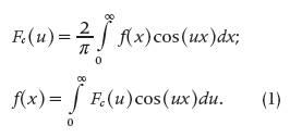
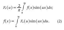
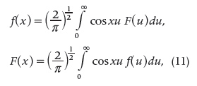
This pair of equations is known today as the forward cosine FT and the inverse cosine FT, respectively. In a similar way, in [12, p. 445] he derived the forward sine FT and the inverse sine FT, that is,

If f is a suitable function defined on the whole real line and is complex-valued, then its forward and inverse FT are respectively and commonly defined as [13, pp. 1–2], that is,

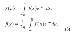
These formulae imply that f admits a representation of the form

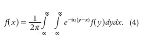
Such representation of the function f, called the Fourier theorem, was first derived by the French mathematician Augustine Louis Cauchy (1789–1857) sometime between 1822 and 1823 and published in 1827 [14, p. 302].
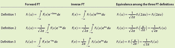
Despite the increasing number of applications of the FT, there is not yet an agreement about the definition of the forward and inverse FT. This disagreement comes from the many ways that (4) can be separated out to form a transform pair of formulae. In fact, depending on the application and the authors, three definitions are used [15, p. 7].
In a more general sense, comparing the formulae in (3), these definitions may also be derived from the following expressions, which in part are defined by [16, p. 182]:

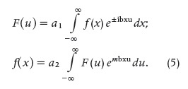
The ± sign and its inverse m in the exponential functions mean that if “+” (or “-”) is chosen in the forward FT, then “-” (or “+”) must be used in the inverse formula. If the same signs are chosen in the forward and inverse formulae, it may be shown that one formula is not exactly the inverse of the other one. In addition, the constant b may take values of either one or 2π, while a1 and a2 are constants, such that a1 • a2 = 1/2π. (See Table 1.)
[accordion title=”Table 1. Three Forward and Inverse FT Definitions.”]

[/accordion]
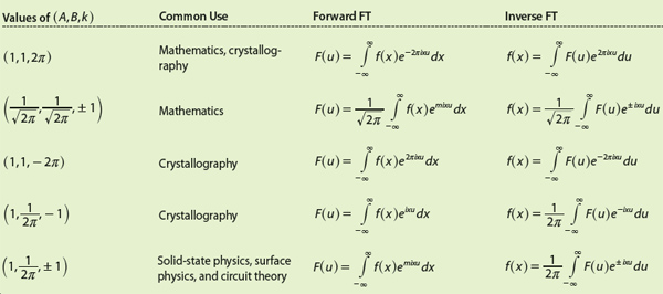
In the first decade of this century, a variation of (5) was presented by Prof. Jirí Komrska of the Brno University of Technology. He pointed out that the following formulae were most common in the physics and mathematics community [17], that is,

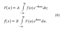
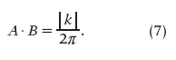
In these formulae, A and B are constants that may be complex; however, if so, the mathematics and proof of some theorems become more difficult, so that often (or almost always) A and B are taken as real positive numbers. In the case of the index k, it must necessarily be a positive or negative real number. Moreover, the link among the three constants has to be such that the following relationship holds:

Specific values of the three constant are given in Table 2. In particular, in solidstate physics and crystallography the different choices of constants required that the definitions of the reciprocal lattices differ by a factor 2π, which caused disputes [18, p. 62].
[accordion title=”Table 2. Definitions of Forward and Inverse FTs in Mathematics and Physics”]

[/accordion]
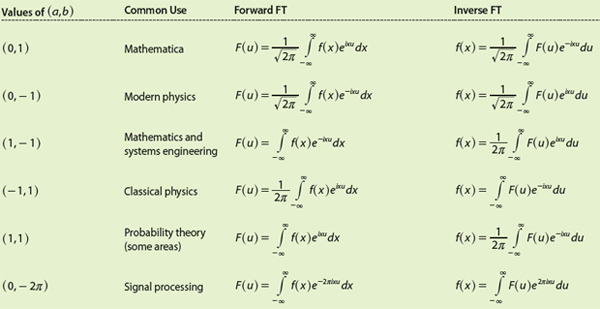
Not long ago, a more complex form of the forward and inverse FT formulae (perhaps even more precise for specific scientific and engineering areas) was given in [19, pp. 1210–1211]. If a and b are real numbers with b ≠ 0, then the FT formulae become

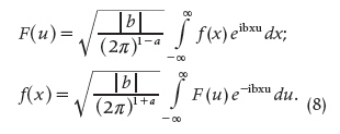
The most common values for a and b and their uses in different areas are given in Table 3.
[accordion title=”Table 3. Definitions of the Forward and Inverse FTs and Areas Where They Are Used”]

[/accordion]
As may be deduced from the previous discussion, the use of any of the definitions given in Tables 1–3 depend on the user’s preferences as well as the specific area of application. Moreover, using a specific definition does not change the essence of the FT formulae, as in any case, properties are the same for any definition and the particular results are essentially equivalent. In other words, as Lewis says [19, p. 1211]:

…[t]here is no real difference between these choices in the sense that there are no important theorems that hold with one choice of (a,b) but not with another.

The only requirement for specific definitions of the FT formulae is to be consistent with them; that is, once one definition is chosen, then it has to be preserved in the derivation of results as well as in the applications.

Genesis of the Term FT

In the 19th century and in the mathematical literature, the term transform has several meanings. Some meanings are related to a change of variable, while others refer to integral representations of functions, as described in [6, p. 355]. Specifically, the first time the word transform was used in the sense that is known today occurred in 1822 [12, §415, p.546]. In fact, the following quotation is found in this that work:

Il est nécessaire d’examiner avec soin la nature des propositions générales qui servent à transformer les fonctions arbitraires: car l’usage de ces théorèmes est très-étendu, et l’on en déduit immédiatement la solution de plusieurs questions physiques importantes, que l’on ne pourrait traiter par aucune autre méthode.

[It is necessary to carefully examine the nature of the general propositions used to transform the arbitrary functions: for the use of these theorems is very extensive, and we immediately derive the solution of many important physical problems, that could not be treated by any other method.]

Moreover, in §419, Fourier again addressed the concept of transform [12, p.559]:

On voit que, dans le second membre de l’équation

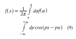
la fonction f(x) est tellement transformée que le signe de fonction f n’affecte plus la variable x mais une variable auxiliaire α. La variable x est seulement affectée du signe cosinus.

[We see that, in the second member of (9) the function f(x) is so transformed that the symbol of the function f no longer affects the variable x, but an auxiliary variable α. The variable x is only affected by the symbol cosine.]

Almost a century after Fourier’s book, the term transformée de Fourier was used for the very first time. It occurred in 1915, in an article written by the Swiss mathematician Michel Plancherel (1885–1967) [20]:

Nous nommerons F(x) la transformée de f(x). Réciproquement, la Transformée de Fourier de F(x) n’est autre que f(x).

[We will name F(x) the transform of f(x). Conversely, the FT of F(x) is none other than f(x).]

However, the term used by Plancherel does not correspond to its modern use because it applies only to those cases in which f is produced from F by the same integral operator that gives F from f.
The next time the term appeared in the literature occurred in 1923, with an article written by the British mathematician Edward Charles Titchmarsh (1899–1963) [21]:

The notion of [FTs] arises from Fourier’s integral formula

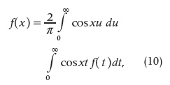
which gives the reciprocal relations

connecting two functions f(x) and F(x). Each of the functions so related is said to be the [FT] of the other.

As the reader may notice in this quotation, Titchmarsh attached the name FT to what today is known as the cosine FT. In the same sense, later in 1923, Titchmarsh authored another article where the term appeared as the main title [22]. Both articles were influential for the use of the term since in those years Titchmarsh started to become an authority in mathematical analysis.
The definitive and modern meaning of the term came from two mathematicians, the American Norbert Wiener (1894–1964) and the English Raymond Edward Alan Christopher Paley (1907–1933), and can be dated as late as 1933 or early as 1934 [23, p. 2]. Finally, a curious note regarding the term transform is found in the book by Bochner [9, p. 222]:

The name transform goes back […] to Cauchy (see Burkhardt, p. 1098), although Cauchy speaks of the “reciprocal” function” rather than the transform.

The book cited by Bochner is [8]. In it, it is quoted that Cauchy defined in [24] that two functions, f and φ, are called “fonctions réciproques de première espèce” (reciprocal functions of the first type) if they are related by what is today called cosine FT (1). Moreover, Cauchy also designated that f and φ are called reciprocal functions of the second type if they are related by what is today called sine FT (2). Hence, the citation by Bochner is not true.

The Earliest Accounts and Books on the FT

The first book that presented the FT theory was, as previously discussed, by Fourier himself [12]. The next account appeared 11 years later, in 1833; its author was the German mathematician Johann August Grunert (1797–1872) [25, §57–60, pp. 273–283]. In 1836, a second account appeared in the British literature, in a book dealing with differential and integral calculus written by the mathematician Augustus de Morgan (1806–1871) [26].
The first textbook exclusively concerning the theory of the Fourier series and integrals was written by German mathematician Oscar Xaver Schlömilch (1823–1901). In this book [27], Schömilch starts to develop the theory of the FT in Chapter II (pp. 72–195). This book has been recognized by Bochner as [9, p. 219]

…the earliest textbook concerning Fourier integral (and in certain respects the only one up to 1931).

Schlömilch’s book has been very influential in the literature; almost any book dealing with Fourier series and transforms follows a similar content and structure. An example is a book by the Bavarian mathematician Martin Ohm (1792–1872), published four years later in Nürenberg [28, p. 358].
Even in the first 30 years of the 20th century, books on the topic adhered quite closely to Schlömilch’s, as it is shown in works by the Scottish mathematician Horatio Scott Carslaw (1870–1954) [29] and by the British mathematician Albert Eagle, published in 1925 [30]. (As an addendum, it can be said that no birth or death dates are reported for Eagle, although it is known that he was a professor of mathematics at Manchester University.)
It is important to mention the marvelous account of the Fourier integral written by Burkhardt [8], which is one of the main sources for tracing back the history of the FT. As curious note, this work was never seen by its author since Burkhardt died on 2 November 1914, two years before the publication of his account.
In 1925, Norbert Wiener gave the first complete and modern treatment of FT [31]. Wiener also exposed the power, extension, and interpretations in the physical sciences of the FT theory in a very long article published in 1930 [32].
In the third decade of the 20th century, the FT theory became a topic of research for many mathematicians and applied scientists and led to four of the most celebrated books: Bochner in 1932 [9], Wiener in 1933 [33] (which includes the results of [31], [32]), Paley and Wiener in 1934 [23], and Titchmarsh in 1937 [34].

The Story of the Fourier Theorem

Since complex-valued functions were not common in Fourier’s time, his book [12] considered only real-valued functions and not the complex-valued functions that are common nowadays. This is also reflected in Schlömilch’s book [27]. This means that only the real part of formula (4) appeared in this book:

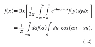
The last equality was completely discovered by Fourier, appearing for the first time in [11]; that is why this formula is known as “Fourier integral” or “Fourier theorem.” This is not the case of Fourier series, which was known and used by other mathematicians beginning in the 18th century. However, Fourier was the first applied mathematician to exploit its nature.
Independently, Cauchy derived (12) in a text published in 1815 [35, pp. 179 and 302]. One year later (1816), the French mathematician Siméon Denis Poisson (1781–1840) published a text in which a similar expression appeared [36, p. 85].
The year 1831 was of great importance for the expression (12) because it was then that the French mathematician Joseph Liouville (1809–1882) coined the expression “Théorème de Fourier,” even though he used it referring to Fourier series instead of to the Fourier integral [37, p. 124]. It was four more years before this term was extended to the Fourier integral. In fact, its first occurrence was in 1835 in an account of fractional differential calculus also written by Liouville [38, p. 226]. Before him, no author used a specific name for (12). For example, in the same year (1835), Poisson reproduced (12) on p. 205 of his book about the theory of heat [39] but only attributed its analysis to Fourier and did not attach to it any specific name. One year later, in 1836, the expression (12) and its denomination appeared in the British literature for the first time in a book about differential and integral calculus written by De Morgan [26, p. 618]. The mention given by De Morgan in his book has historical importance since it seems that the theorem was already known in British mathematical circles. In fact, he wrote,

…by the definition of a definite integral,

a result which is usually called Fourier’s theorem.

The consolidation of (12) and its denomination was quite fast in mathematical circles such that its first appearance in an encyclopedia occurred in 1838 [40], where on p. 390 it can be read:

In the (Théorie de la Chaleur), the object of which is the deduction of the mathematical laws of the propagation of heat through solids, Fourier extended the solution of [PDEs], gave some remarkable views on the solution of equations with an infinite number of terms, expressed the particular value of a function by means of a definite integral containing its general value (which is called Fourier’s theorem).

Five years later, in 1843, there was an active use of Fourier’s results in England. In fact, in this year and in the same journal, three articles appeared about them. The first one was about the motion of heat in a sphere [41], the second one was about the use of the theorem in describing the vibration of cords [42], and the third one concerned the demonstration of the theorem under particular conditions [43].
Even when De Morgan had used the name Fourier theorem when referring to (12), he also used the term Fourier integral, as reflected in his article published in 1848 [44]. Specifically, on p. 191 he wrote,

In the German literature, (12) appeared in a workbook about pure mathematics published in 1833 by Grunert [25]. In §57–60 (pp. 273–283), Grunert made a derivation of the Fourier integral from the Fourier series and computed some values of definite integrals from it. In a similar way, a second explicit reference and complete treatment of (12) was given by Schlömilch in his book [27].
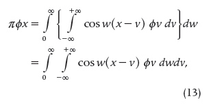
Finally, a curious and incorrect observation concerning (12) was made by the Italian mathematician and historian Umberto Bottazzini (1947) [47, pp. 78–79]:

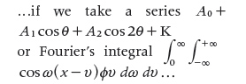
In the Théorie analytique, Fourier went on to consider the problem of propagation of the heat in solid homogenous bodies, such as rings, spheres, cylinders, cubes, etc. By studying the propagation along an infinite line, he showed how a function can also be represented in the following manner:

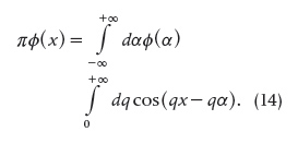
This representation of φ(x) by means of integrals, as Fourier himself admitted, had been unknown to him in 1807, when he presented his first article on the propagation of heat to the Institute. He first found it two years later, in a article that Laplace published in the Journal de l’École Polytechnique in 1809.

However, after a revision was made to Fourier’s book [12], in §364 it is found that the equation attached to Laplace was

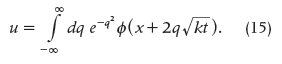
In fact, Fourier wrote [12, p. 454]:

…et la valeur de u satisfera nécessairement à l’équation

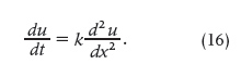
Cette intégrale, qui contient une fonction arbitraire, n’était point connue lorsque nous avons entrepris nos recherches sur la théorie de la chaleur, qui ont été remises à l’Institut de France dans le mois de décembre 1807: Elle a été donnée par M. Laplace, dans un ouvrage qui fait partie du tome VI des Mémoires de l’école polytechnique; nous ne faisons que l’appliquer à la détermination du mouvement linéaire de la chaleur.

[… and the value of u will necessarily satisfy (16). This integral which contains one arbitrary function was not known when we had undertaken our researches on the theory of heat, which were transmitted to the Institute of France in the month of December 1807: it has been given by M. Laplace, in a work which forms part of volume VIII of the Mémoires de l’École Polytechnique; we apply it simply to the determination of the linear movement of heat.]

The article written by the French mathematician Pierre-Simon Laplace (1749–1827) and cited by Fourier is [46]. Thus, Bottazzini’s quotation is certainly incorrect.
As an additional note, readers interested in tracing back the first proofs of (12) should read the historical article by the Italian mathematician Silvia Annatarone [47]. As a further remark, most of these proofs consider the use of convergence factors of the exponential type, a technique commonly used to reduce the so-called Gibbs phenomenon, which consists of an overshoot of the approximating function to the original one near a point of discontinuity.

The Origin of the FT of Derivatives and Indefinite Integrals

One of the most important results in the application of the FT to solve DEs in science and engineering is that, for a positive integer number n, an nth order ordinary DE with constant coefficients is Fourier transformed into an nth degree algebraic equation. In addition, it allows transforming any PDE with constant coefficients into an ordinary DE with constant coefficients. This is because the FT of an nth derivative of a suitable realvalued function f(x), with FT F(u), is given by (iu)^n F(u), with i^2 = -1.
This result was discovered exclusively by Fourier when the number n is even (a multiple of two or four), and it is described in his book [12, p. 543]. The way Fourier expressed his result is by using the corresponding formula similar to (12); that is, (in modern notation),

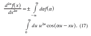
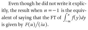
In (17), the positive sign is chosen when n is even; otherwise, the negative sign is chosen (when n is odd). Fourier went further and said that if the same rule is followed relative to the choice of sign, then

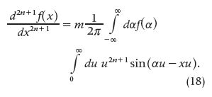
Moreover, he made the point that integration of the third member of (12) several times with respect to x results in writing in front of the symbol sine or cosine a negative power of u.

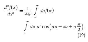
The generalization of expressions (17) and (18) was given by Fourier a few pages further on. In fact, on pp. 561–562 of [12], he wrote that if n is any positive or negative integer number, then

Tracing Back the History of the FT Eigenfunctions and Eigenvalues

As an introductory note to this section, recall that the word eigenvalue comes from the German eigenwert, which means proper or characteristic value, while eigenfunction is from eigenfunktion, meaning proper or characteristic function. These concepts from linear algebra define that, for a given square matrix A, if there are values of the variable λ for which nonzero solutions can be obtained (that is,

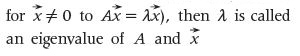
corresponding eigenvector. It is important to underline that in order for λ to be an eigenvalue, it is essential to find nonzero solutions to the equation.

Extending these concepts, an interesting question about the FT is whether there is a nonzero function f(x), or a set of such functions, which after obtaining the FT F(u) results in a proportion of

If such a function exists, then it is called a FT eigenfunction with FT eigenvalue λ. Notice that (20) implies that the function is shape-invariant under the FT; moreover, it also implies that there is no dilation in the variable u. One example of this class of functions

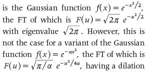
in the variable u. In this way, this function cannot be considered an eigenfunction of the FT.

The first time that the Gaussian function

was considered as an eigenfunction of the FT occurred in an article by Wiener published in 1929 [48]. This mathematician later reconsidered and complemented his own results in a book [33].

It was not until 1991 that M.J. Caola described a method to generate a function having a FT as the function itself from another arbitrary Fourier transformable function [49]. This article by Caola and those by Soares et al. [50], Vaidyanathan [51], Horikis and McCallum [52], and McCallum and Horikis [53] are the origin of the main methods to generate the FT eigenvalues and eigenfunctions.

Final Words by Fourier Himself and Other Authors

The foundations of the FT theory appeared for first time in Fourier’s work submitted to the Institute de France. Its applications opened a new way of understanding many physical phenomena. Even for Fourier, his theory was a surprise. At the beginning of his book [12, §428, p.580], the following statement is found, where he suggests he regarded the transformations as otherwise useless:

Les intégrales que nous avons obtenues ne sont point seulement des expressions générales qui satisfont aux équations différentielles: Elles représentent de la manière la plus distincte l’effet naturel, qui est l’objet de la question. C’est cette condition principale que nous avons eue toujours en vue, et sans laquelle les résultants du calcul ne nous paraitraient que des transformations inutiles.

[The integrals we have obtained are not only general expressions that satisfy the DEs; they represent in a different way the natural effect, which is the object of the problem. This is the main condition that we have always had in view, and without which the results of the operations would appear useless transformations.]

Many authors have written about general integral transforms; however, their importance and comparison with the invention of logarithms is best expressed on p. 1 of the book by Miles [54]:

The introduction of an integral transform in a particular problem may be advantageous if the determination or manipulation of the transform is simpler than the function itself, much as the introduction of log x in place of x is advantageous in certain arithmetical operations.

The way Fourier derived (1) and (2), or equivalently (3), has been similar since then. These are derived from Fourier series by extending the idea to functions defined on the whole real line. However, as Papoulis mentions [13, pp. 1–2]:

The validity of the expansions of the form (3) is often established from a related result in Fourier series. However, this approach is not always mathematically satisfactory. Theoretically, it does not give the conditions for the validity of (3) and is based on a limited interpretation of the meaning of an integral.

In the same sense, the French mathematician Jaques Arsac (1929–2014) points out that such a derivation from Fourier series [55, p. 49]

…does not constitute a proof and has only a formal value. On the other hand, it assumes a previous knowledge of the terms in the Fourier series and the value of this approach seems doubtful.

The FT of a function is a precise function defined by the integral and nothing more.
The FT theory exists by its own right, with or without the existence of Fourier series. However, it is important to mention that most of the results associated with the FT are extensions or analogies of those corresponding to the Fourier series. Scientists and applied mathematicians have considered the Fourier series as a point of reference for the development of the FT. However, not all of the results of the FT are analogous in Fourier series; this is the case of the following example, which has no place in the series form:

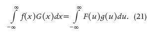
Here, functions F and G are the FTs of functions f and g respectively.

References

1. M. S. Klamkin and D. J. Newman, “The philosophy and applications of transform theory,” SIAM Rev., vol. 3, pp. 10–36, 1961.
2. M. A. B. Deakin, “Euler’s invention of the integral transforms,” Arch. Hist. Exact Sci., vol. 33, pp. 307–319, 1985.
3. I. N. Sneddon, Use of Integral Transforms. New York: McGraw-Hill, 1972.
4. M. A. B. Deakin, “Euler´s version of the Laplace transform,” Am. Math. Mon., vol. 87, no. 4, pp. 264–269, 1980.
5. M. A. B. Deakin, “The development of the Laplace transform, 1737–1937: I. Euler to Spitzer, 1737–1880,” Arch. Hist. Exact Sci., vol. 25, no. 4, pp. 345–390, 1981.
6. M. A. B. Deakin, “The development of the Laplace transform, 1737–1937: II. Poincaré to Doetsch, 1880–1937,” Arch. Hist. Exact Sci., vol. 26, no. 4, pp. 351–381, 1982.
7. M. A. B. Deakin, “The ascendancy of the Laplace transform and how it came about,” Arch. Hist. Exact Sci., vol. 44, no. 3, pp. 265–286, 1992.
8. H. F. Burkhardt, “V. Das Fouriersche Integral,” in “Trigonometrische reihen und integrale (bis etwa 1850),” in Encyklopädie der mathematischen Wissenschaften mit Einschluss ihrer Answendungen, vol. II, H. F. Burkhardt, M. Wirtinger, R. Fricke, and E. Hilb, Eds. Leipzig: Druck und Verlag von B. G. Teubner, 1904–1916, pp. 1085–1173.
9. S. Bochner, Vorlesungen über Fouriersche Integrale. Leipzig: Akademische Verlagsgesellschaft, 1932.
10. J. B. J. Fourier, Théorie de la propagation de la chaleur dans les solides, Manuscrispt submitted to the Institute of France, 21 Dec. 1807.
11. J. B. J. Fourier, “Théorie du mouvement de la chaleur dans les corps solides,” Mémoires de l’Académie royale des sciences de l’Institute de France, no. 4, 1811.
12. J. B. J. Fourier, Théorie analytique de la chaleur. Paris: Chez Firmin Didot, Père et Fils, 1822.
13. A. Papoulis, The Fourier Integral and Its Applications. New York: McGraw-Hill, 1962.
14. A. L. Cauchy, “Théorie de la propagation des ondes a la surface d’un fluide pesant d’une profondeur indéfinie, Note XIX, Sur les fonctions réciproques,” Mémoires présentés par divers savants á l’Académie Royale des Sciences de l’Institut de France et imprimés par son ordre. Sciences mathématiques et physiques. Tome I. Imprimé par autorisation du Roi a l’Imprimerie royale; 1827. OEuvres Complètes d’Augustin Cauchy, Series 1, Tome 1, 1882.
15. R. N. Bracewell, The Fourier Transform and Its Applications (3rd ed.). New York: McGraw-Hill, 1999.
16. J. D. Gaskill, Linear Systems, Fourier Transforms and Optics. New York: John Wiley, 1978.
17. J. Komrska, Fourierovské metody v teorii difrakce a ve strukturni analýze. Brno: Akademické nakladatelsví CERM, 2007.
18. C. Kittel, Introduction to Solid State Physics (4th ed.). John Wiley: New York, 1971.
19. A. D. Lewis. (2015, May 15). A Mathematical Introduction to Signals and Systems: Time and Frequency Domain Representations of Signals, vol. II. [Online].
20. M. Plancherel, “Sur la convergence et sur la sommation par les moyennes de Cesàro de f (x)cos xydx. z a z lim “3 # ” Math. Ann., vol. 76, pp. 315–326, 1915.
21. E. C. Titchmarsh, “Hankel transforms.” Proc. Camb. Philos. Soc., vol. 21, pp. 463–473, 1923.
22. W. C. Titchmarsh, “A contribution to the theory of Fourier transforms.” Proc. Lond. Math. Soc., Series 2, vol. 23, pp. 279–289, 1923.
23. R. E. A. C. Paley and N. Wiener, Fourier Transforms in the Complex Domain. Providence: American Mathematical Society, 1934.
24. A. L. Cauchy, “Sur une loi de réciprocité qui existe entre certaines fonctions.” Bulletin des Sciences par la Société Philomathique de Paris, pp. 121–124, 1817.
25. J. A. Grunert, Wörterbuche der reinen mathematishes. Supplemente zu Georg Simon Klügel’s. Leipzig: E. B. Schwickert Verlag, 1833.
26. A. De Morgan, The Differential and Integral Calculus. London: Baldwin and Cradock, 1836.
27. O. X. Schlömilch, Analytische studien: die Fourier’schen reihen und integrale, vol. 2. Leipzig: Verlag von Wilhem Engelmann, 1848.
28. M. Ohm, Versuch eines vollkommen consequenten Systems der Mathematik: Die Auswerthungs bestimmter Integrale, so wie die Theorie der Reihen und der Integrale des Fourier, vol. 9. Nürnberg: Friedrich Korn, 1852.
29. H. S. Carslaw, An Introduction to the Theory of Fourier’s Series and Integrals and the Mathematical Theory of the Conduction of Heat. London: MacMillan & Co., 1906.
30. A. Eagle, A Practical Treatise on Fourier’s Theorem and Harmonic Analysis for Physicists and Engineers. New York: Longamans, Green and Co., 1925.
31. N. Wiener, “On the representation of functions by trigonometric integrals,” Math. Z., vol. 24, pp. 575–617, 1925.
32. N. Wiener, “Generalized harmonic analysis.” Acta Math., vol. 55, pp. 117– 258, 1930.
33. N. Wiener, The Fourier Integral & Certain of Its Applications. Cambridge, U.K.: Cambridge Univ. Press, 1933.
34. E. C. Titchmarsh, Introduction to the Theory of Fourier Integrals. Oxford, U.K.: Oxford Univ. Press, 1937.
35. A. L. Cauchy, “Théorie de la propagation des ondes a la surface d’un fluide pesant d’une profondeur indéfinie (Prix d’analyse mathématique, Concours de 1815 et de 1816),” Mémoires de l’Académie Royale des Sciences de ‘Institut de France, Classe des Sciences Mathématiques et Physiques, 1 [OEuvres Complètes, 1er Série, Tome 1 (1882), Paris, France: Gauthier-Villars].
36. S. D. Poisson, “Mémoire sur la théorie des ondes,” Mémoires de l’Académie Royale des Sciences de l’Institut de France, 1816.
37. J. Liouville, “Mémoire sur le calcul des différentielles à indices quelconques,” J. de l’École Polytechnique. Vingt-uniéme Cahier, Tome XIII, pp. 71–162, 1832.
38. J. Liouville, “Mémoire sur l’usage que l’on peut faire de la formule de Fourier, dans le calcul des différentielles à indices quelconques,” J. für die Reine und Angew. Math., Dreizehnter Band, pp. 219–232, 1835.
39. S. D. Poisson, Théorie mathématique de la chaleur. Traité de Physique Mathématique. Paris: Imprimerie de Bachelier, 1835.
40. The Society for the Diffusion of Knowledge, The Penny Cyclopaedia, vol. X. London: Charles Knight and Co., 1838.
41. By a correspondent, “Note on a passage in Fourier’s heat,” Camb. Math. J., vol. III, pp. 25–27, 1843.
42. “Note on vibrating cords,” Camb. Math. J., vol. III, pp. 257–258, 1843.
43. “On Fourier’s theorem,” Camb. Math. J., vol. III, pp. 288–290, 1843.
44. A. de Morgan, “On divergent series and various points connected with them,” Trans. Camb. Philos. Soc., vol. 8, pp. 182–203, 1848.
45. U. Bottazzini, The Higher Calculus: A History of Real and Complex Analysis from Euler to Weierstrass. New York: Springer- Verlag, 1986.
46. P. S. Laplace, “Sur les intégrales définies des équations à différences partielles,” J. de l’École Polytechnique. Tome VIII, XVe Cahier, pp. 235–244, 1809.
47. S. Annaratone, “Les premières démonstrations de la formule intégrale de Fourier,” Rev. d’histoire des Math., vol. 3, pp. 99–136, 1997.
48. N. Wiener, “Hermitian polynomials and Fourier analysis,” J. Math. Phys., vol. 8, pp. 70–73, 1929.
49. M. J. Caola, “Self-Fourier functions,” J Phys. A Math. Gen., vol. 24, pp. L1143–L1144, 1991.
50. L. R. Soares, H. M. Oliveira, R. J. S. Cintra, and R. M. Campello de Souza, “Fourier eigenfunctions, uncertainty Gabor principle and isoresolution wavelets,” XX Simpósio Brasileiro de Telecomunicaçoˉes-SBT’03. Rio de Janeiro, Brasil, 2003.
51. P. P. Vaidyanathan, “Eigenfunctions of the Fourier transform,” Inst. Electron. Telecomm. Eng. J. Educ., vol. 49, pp. 51–58, 2008.
52. T. P. Horikis and M. S. McCallum, “Self-Fourier functions and the self- Fourier operators,” J. Opt. Soc. Am., vol. 23, pp. 829–834, 2006.
53. M. S. McCallum and T. P. Horikis, “Selftransform operators,” J. Phys. A Math. Gen., vol. 39, pp. L395–L400, 2006.
54. J. W. Miles, Integral Transforms in Applied Mathematics. Cambridge, U.K.: Cambridge Univ. Press, 1971.
55. J. Arsac, Fourier Transforms and the Theory of Distributions. Englewood Cliffs, NJ: Prentice Hall, 1966.