Deconvolution

Mathematics does not really exist, for it is a creation of the Human Mind, and, in that respect, it approaches a Supreme Idea, as some kind of Divine Enlightenment.
The origins of convolution and its further and rather complex historical development were dealt with in detail by Alejandro Domínguez in a previous article [1]. We saw there that it can be traced back to the middle of the 18th century; however, its modern form and use are not more than 50 or 60 years old.
The present article addresses its inverse operation, i.e., deconvolution, approachable in both the continuous area and the discrete field. Because convolution is sometimes referred to as convolution product by using the asterisk symbol (*), in a similar spirit the term deconvolution quotient might be suggested with the symbol

so that as e(t)*w(t) represents convolution of the indicated functions, e(t)*/*w(t) would represent their deconvolution, implying some kind of convolution division.
Not infrequently, solutions to equations in continuous mathematics may become very difficult, even intractable. Fortunately, our computer age permits, in the discrete field, the solving of anything, no matter how complex and/or long the calculations may be. In addition to the “continuous” versus “discrete” controversy that may arise due to philosophical trends when searching for the perfect exact solution, and rejecting numerical approximations as mathematical sins, the truth is that any inverse algorithm is in itself ambiguous: say, the simple difference (a – b), as opposed to the algorithm of the sum, may produce imperfect results, as (1 – 0.33333); or division, as the inverse of multiplication, when, for example, dividing 10 by 3; or the square root (with its double sign), as the counterpart of x². Deconvolution is no exception in this respect, and its indeterminations, when continuous, may lead to essential dead ends or, when discrete, become extremely annoying with almost useless results.

The Concept of Deconvolution

Deconvolution had a relatively early application in seismology, when in 1950 Enders Robinson, a graduate student at the Massachusetts Institute of Technology, was working on the seismogram. He assumed that the recorded seismogram s(t) is the convolution of an earth-reflectivity function e(t) and a seismic wavelet w(t) from a point source, where t is the recording time. Thus, the convolution equation would be

Seismologists want to obtain the reflectivity e(t), which contains information about the earth’s structure. Equation (1), by application of the convolution theorem, can be treated with the Fourier transform to become

in the frequency domain. The reflectivity may be recovered by shaping the estimated wavelet to a spike, somewhat similar to a Dirac delta function. It is not rigorous, but the result may be seen as

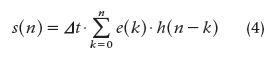
where N is the number of reflection events, τi the reflection times of each event, and ri the reflection coefficients.
The foundations for deconvolution and time-series analysis were largely laid later on by Norbert Wiener, based on work he had done during World War II (1939–1945) that had been classified at the time. Perhaps Robinson and Wiener worked together, although we could not assert it. Other early attempts to apply these theories occurred in the fields of weather forecasting and economics [2].
Let us now focus on the present objective: to partially review the mathematics supporting discrete deconvolution (DD), as well as its applications in physiology, while trying to foresee what its prospects are from the point of view of bioengineering. A comment must be added here: because convolution is also a process that filters out signals, deconvolution can be seen as a reconstruction operation on those signals.

The Mathematics of Deconvolution

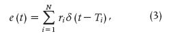
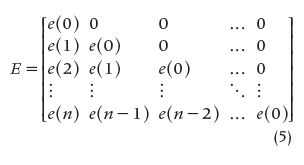
There are two ways to approach DD: in the time domain and in the frequency domain. In this article, we restrict ourselves to the time domain. For that matter, let us write the discrete form of the convolution integral as

where s(n) is the output signal from the studied system, e(n) is the input signal, h(n) represents the system’s impulse response, and Δt is the sampling interval. Equation (4) can be written as the triangular matrix E, called the input matrix. The two column matrices E and S can also be set in such a way that the whole group of matrices represents a discrete approximation of convolution and deconvolution, respectively, where E^-1 stands for the inverse of E and the three signals are created by adequate sampling of the respective continuous versions with a sampling interval equal to Δt. That is,

and

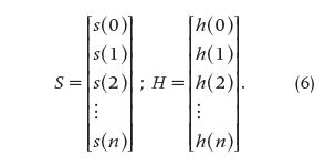
The equations that follow [(7) and (8)] represent a discrete approximation of convolution and deconvolution, respectively, making use of the matricial notation, where E^-1 is the inverse of the matrix E, i.e.,

and

It must be stressed that two parameters are important, i.e., the initial signal value (which determines whether the matrix can be inverted) and the sampling frequency (which determines the resolution, in turn, related to Δt).

How the Matrix DD Method Can Be Tested

First, applying different known inputs checks the respective outputs. Thereafter, noise is superimposed to see how the new outputs are affected. Using a computer, a linear system showing the impulse response described by (9) was simulated as

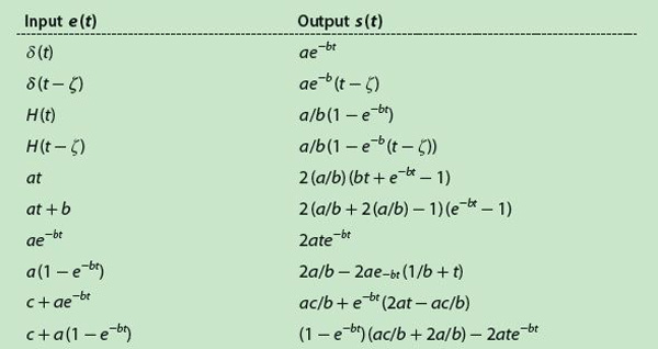
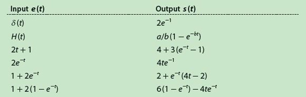
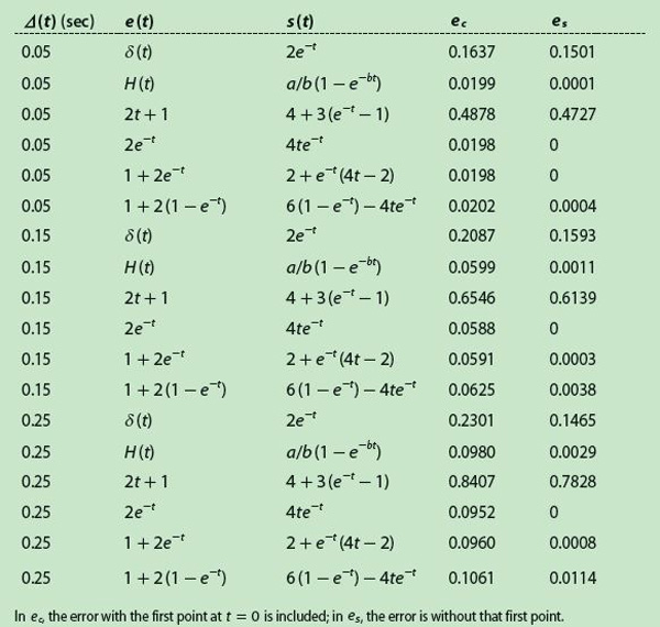
Table 1 displays a collection of several wel l-known input signals and their respective outputs calculated by continuous convolution, which involves more or less simple mathematical operations. The input δ(t) is the Dirac delta function, and H(t) is the standard unit step. However, the method cannot resolve situations where the signal value is zero at t = 0 because the matrix E is triangularly inferior, i.e., the elements of its diagonal are its eigenvalues and, in such a case, these values are zero, making the matrix noninvertible. Hence, Table 1 is reduced to the values in Table 2, with only six pairs of functions.
[accordion title=”Table 1. Pairs of Known Input-Output Signals.”]

[/accordion]
[accordion title=”Table 2. Final Input-Output Signal Pairs.”]

[/accordion]
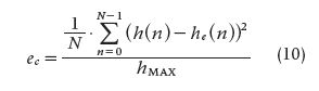
In Table 2, the generic constants have been replaced by arbitrarily chosen numerical values, i.e., a = 2, b = 1, c = 1, and ζ = 5. By means of (9) and using the functions of Table 2, the method was simulated with Δt = 5 seconds. Furthermore, a sampling frequency must be selected to pick up the samples from the continuous functions; thus, several sampling periods were tested. Except for the δ(t), everything was simulated with Matlab. For the delta function, instead we used a model based on partial sums, as described by Fejér in the early 1900s [3], [4]. The error produced after estimating the impulse response is obtained with

and

Both (10) and (11) describe the mean squared error (MSE) normalized to the maximum impulse response value. In these equations, ec refers to the MSE when the first point at t = 0 is taken into account, and es refers to MSE without considering that first point. From Tables 1 and 2, the best input-output combination was chosen using as a criterion the smallest estimated error in the absence of noise. For that matter, Gaussian noise (μ = 0; σ = 10% of the signal value) was added to the input signal for the purpose of checking the method’s performance.
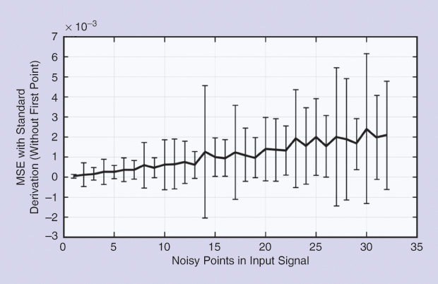
For the simulation, noise was added at each iteration, increasing by one point for each case: in other words, adding noise to one point, two points, three points, and so on. The calculation was carried out with 100 samples per iteration. For each of these, MSE was computed, as defined by (10) and (11). Thereafter, errors were averaged out along with the standard deviations (SDs), so that two curves were obtained for the MSE: one considered the first point and another did not.

Test Results

[accordion title=”Table 3. MSE as a Function of the Sampling Interval”]

[/accordion]
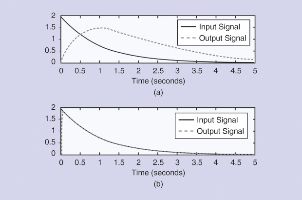
Table 3 shows the results obtained normalizing the MSE for different sampling frequencies. The numerical values seem to confirm an intuitive idea, i.e., increasing the sampling frequency resulted in decreasing the error of the estimated impulse response. Moreover, the MSE grows significantly when the first point is included, and that appears to be a problem inherent to the method because the initial value depends linearly on the output signal at that particular instant zero.
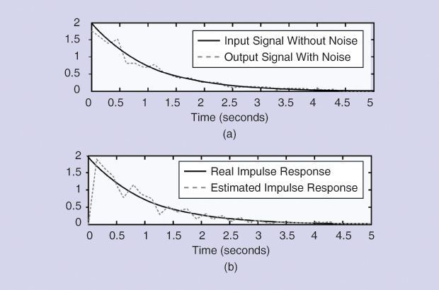
Thus, if the input starts with a null value, the estimated impulse response will also be zero, introducing an important error in most cases (Figure 1). Noise was added to the input, producing the behavior of the normalized MSE displayed in Figures 2 and 3, where the number of points appears on the horizontal axes. Figure 2 shows the results when noise was added to the input signal, sampling time was 0.15 seconds, and the point at zero time was not considered.

Applications in Physiological Systems

Renography

A nuclear renogram is performed by injecting a radioisotope into a vein. The isotope then flows through the blood vessels of the kidneys and is filtered by the glomeruli and/or secreted at the renal tubules. As the isotope flows into the collecting system, it is detected by a nuclear camera placed behind the kidneys. The amount of isotope filtered and drained by the kidneys, in counts per second, produces a collection of points as time proceeds, thus giving graphic information regarding drainage from the kidneys (the socalled retention function, because it tells how long the kidneys retain the foreign substance; this is also related to the residence time of the substance).
A renogram produces data useful for detecting obstructions, compromised blood flow, or the function of one kidney relative to the other or to a normal organ. Hence, renography is a dynamic study where time is an important dimension for kidney function evaluation. The upslopes of the curves demonstrate kidney uptake, and downslopes refer to elimination. The two most common radiolabeled pharmaceutical agents used are Tc99m-mercaptoacetyltriglycine (MAG3) and Tc99m-diethylene triamine pentacetic ac id (DTPA). Tc99m-MAG3 is by far a better diagnostic agent than Tc99m- DTPA, particularly in neonates, patients with impaired function, and patients with suspected obstruction.

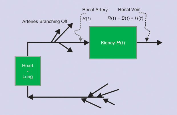
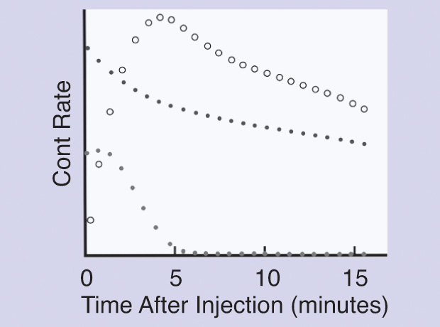
Dynamic renal studies lend themselves to analysis by mathematical DD. The response of a kidney to a bolus injection of radioisotope into the renal artery can be derived from the renogram, which results from the timevarying input of markers from the blood into the kidneys. Figure 4 shows a schematic of the system, and Figure 5 displays the experimental curves, including the result of numerically deconvolving R(t) by B(t). Symbolically, the operation in its two directions could be written as

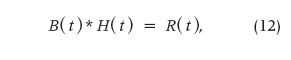
the convolution product, and

the convolution division or deconvolution. The latter operation (13) is the inverse of the former, making use of the proposed notation given previously.

The literature on deconvolution applied to renography, as well as the discussion of its pitfalls, has been extensive since the technique was introduced [5], [6]. Without attempting a complete review, we can note that more than two decades ago, in Barcelona, Spain, transit time and relative kidney function were studied by González et al. [7] using two different tracers. Transit times were on the order of 300 seconds, although the deviations were rather large (on the order of 100 seconds). Other contributions worth mentioning are those by Lawson, Stevens et al., and Thomas et al. [8]–[10]. A 2010 study carried out at the University of Jordan compared matrix inversion deconvolution with the Rutland-Patlak (R-P) plot, which is a very specific method (not described here). The values of the renal parenchymal mean transit time obtained by applying matrix inversion were significantly higher than those obtained using the R-P plot. However, a strong positive correlation was found between the values obtained by applying both methods. These authors believe that R-P analysis is more reproducible than the matrix inversion method because the latter relies heavily on the accuracy of the first point [11].
No doubt, whatever the variants in the approach may be, deconvolution appears to be a useful complementary mathematical tool for renal function analysis, already having over a good 40 years of tests and development.

Gastrointestinal Absorption Kinetics Analyzed by Deconvolution

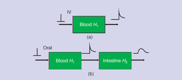
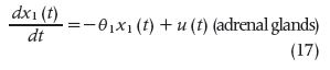
In 1967 in Italy, Giorgio Segre was perhaps the first to report intestinal absorption results obtained from experimental measurements and application using DD [12]. Figure 6 briefly outlines the basic concept, where the intestinal tract is viewed as a transfer system. In Figure 6(a), a sudden infusion of a substance is given intravenously. Thus, it can be regarded as an impulse e(t), introduced in a very short time, like δ(t). The response is r1(t) = h1(t), or the impulse response, with h1 being the blood compartment transfer function. In Figure 6(b), an oral amount e(t), in a way similar to the delta function, of the same substance is ingested by the subject, producing a response r2(t), which should be detected between the first and the second block (obviously impossible to record). This acts as input to the intestines. The final response is r3(t), detectable at the lower right-hand side of the figure. From this, we can determine the following general convolution relationships in the s domain:

and

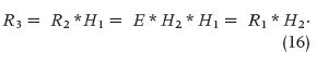
In (14)–(16), the uppercase letters represent, respectively, the Laplace transforms of the time-dependent lowercase- letter variables, and the asterisk (*) is the convolution product. It is clear that deconvolving R3 with R1 would lead to an estimate of the intestinal transfer function H2(s), the impulse response of which is h2(t). Either of these two functions, the first in the s domain and the second in the t domain, quantitatively describes the intestinal kinetics.

Endocrine Impulse Functions and Deconvolution

Several neuroendocrine glands secrete their hormones as short bursts, as well described in many papers, and such bursts can be viewed as physiologically imperfect delta functions. The brilliant concept proposed by Veldhuis, Carlson, and Johnson in 1987, and much improved in 1995, simply said there was no need of an external generator or injection, because the system has its own. Deconvolution did the rest, and a series of superb contributions greatly improved the quantification neuroendocrine process [13], [14]. However, quantitative neuroendocrinology is much more, by far, than deconvolution.
Perhaps Johnson and Velhuis in 1995 [14] characterized best the whole intent in the preface to their outstanding treatise, which we dare to qualify as clearly being within a bioengineering framework:

As experimental strategies have become more sophisticated, highspeed computing has been required for the formulation and solution of more elaborate statements of neuroendocrine pulsatility, such that matrices are needed to handle 100 to 300 equations, each containing 10 to 30 variables. Obviously, neuroendocrinology in its quantitative endeavor appears as a multidisciplinary entity with outstanding contributions from probability theory, systems engineering, stochastic differential equations and the experimental natural sciences such as cell and molecular biology and other approaches to subcellular analyses.

Five of 16 chapters of [14] (that is, 31% of the book) deal with deconvolution analysis based on the burst intrinsic glandular secretion as the delta function simil or S(t), the blood hormonal concentration C(t) as the output signal, and the system elimination function E(t) as the characteristic time-transference function called h(t) in systems engineering. This shows the importance these editors placed on this subject.
It has been suggested that parathyroid hormone (PTH) is secreted in a pulsatile fashion. To characterize PTH secretory dynamics in healthy subjects, seven young women and six young men were studied, all of whom had hip and spine bone densities determined by dual photon densitometry. PTH concentrations were measured by immunoradiometric assay in blood sampled every 2 minutes during the course of 6 hours. Ionized calcium levels were obtained during the second and third hours of the study. Plasma PTH profiles were subjected to deconvolution analysis, which classifies measured hormone levels into secretion and clearance components. Crosscorrelation analysis was performed to assess direct or inverse correlations between serum PTH and ionized calcium concentrations at various time lags. PTH was secreted in a dual fashion, with significant basal (tonic) secretion and PTH pulses occurring approximately every 20 minutes. Pulsatile PTH secretion accounted for ~25% of the total secreted PTH, with no differences between men and women, nor any significant correlations between PTH and ionized calcium concentrations. In 1993, Samuels et al. concluded that in normal subjects, the predominant mode of PTH secretion is tonic, with superimposed PTH pulses having small amplitude but high frequency [15].
Another team investigated daily cortisol production and clearance rates in a group of 18 normal unstressed pubertal males: nine early pubertal and nine late pubertal subjects [16]. Deconvolution analysis was applied to serum cortisol concentrations obtained every 20 minutes for 24 hours. Subject-specific characterization of adrenocortical secretory episodes, cortisol production rate, and serum hormone half-life assessed potential roles of sexual maturation and changing gonadal steroid hormone concentrations on glucocorticoid physiology. No differences were observed between the two groups in secretory burst frequency and half duration, mass of cortisol released per secretory episode, average maximal rate of hormone secretion, and serum cortisol half-life. The investigators concluded that in normal pubertal males, 1) cortisol production rates as estimated by deconvolution analysis are in agreement with other independent isotopic estimates but lower than many previous estimates; 2) the rise in serum gonadal steroid hormone levels is unassociated with alterations in the production rate or metabolic clearance of cortisol; and 3) increased secretory burst frequency, amplitude (maximal rate of cortisol secretion), and mass of cortisol released per adrenocortical secretory episode give rise to the normal diurnal rhythm of circulating cortisol.
Somewhat later, the same team sought to determine whether elevated circulating growth hormone (GH) concentrations in uremic prepubertal children were due to an increase in GH secretory activity by the pituitary gland or a decrease in the metabolic clearance of GH consequent to reduced glomerular filtration rate (GFR) [17]. Deconvolution analysis was applied to the nighttime plasma GH profiles of 11 children with preterminal chronic renal failure, 12 children with end-stage renal disease (ESRD), and a control group of matched children with idiopathic short stature (n = 12). The mean half-life of endogenous GH in children with ESRD and preterminal chronic renal failure was significantly higher than in controls. GH half-life correlated inversely with GFR. The number of GH secretory bursts per 10 hours in children with ESRD was amplified, compared to those with preterminal chronic renal failure and controls. GH production rate varied by a broad range in the three groups. It was highest in the ESRD group, mainly as a result of an increased number of GH secretory bursts, and not statistically different in the group with preterminal chronic renal failure and the controls. Total immunoreactive plasma insulin-like growth factor 1 (IGF-1) levels were indistinguishable among groups. This disruption of the normal relationship between circulating GH and total plasma IGF-1 levels in children with ESRD suggests a relative insensitivity to the action of GH in uremia [17].
In 2011, Hill et al. [18] reported that glucocorticoid replacement therapy uses two or three daily regimens of hydrocortisone (HC) with variable distribution of the dose during the course of the day. Deconvolution analysis determines the mass of hormone that must be secreted to attain a particular serum concentration. These researchers used this methodology to determine the amount and distribution of cortisol during a 24-hour period in 79 adults (41 male) aged 60– 74 years and 30 children (24 male) aged 5–9 years. The subjects underwent 24-hour serum cortisol profiles, with samples drawn at 20-minute intervals. Profiles were subjected to deconvolution analysis using a cortisol half-life of 80 minutes to yield the amount of cortisol released by the adrenal gland to generate the corresponding serum concentration. Cortisol secretion occurred in discrete bursts. Daily cortisol secretion ranged from 5.6–12.4 mg/m²/days in adults and 7.2–16.5 mg/m²/days in children; peak secretion was lower in adults. The team concluded that these observations suggest an optimal dosing and distribution regimen for HC replacement.
The same group of researchers in 2013 [19] reported that HC therapy is based on a dosing regimen derived from estimates of cortisol secretion, but little is known of how the dose should be distributed throughout the 24 hours. Again, by means of deconvolution analysis, the team obtained HC dosing schedules in young children and older adults. Data were apparently obtained from the same group of patients participating in [18]. Mean daily cortisol secretion was similar between adults and children, but peak serum cortisol concentration was higher in children compared with adults. The authors concluded that these observations suggest that the daily HC replacement dose should be equivalent, on average, to 6·3 mg/m2 body surface area per day in adults and 8·0 mg/m2 body surface area per day in children. Differences in distribution of the total daily dose between older adults and young children must be taken into account when using a three or four times daily dosing regimen.
A significant paper by Faghih and his group in 2014 [20] dealt with deconvolution of serum cortisol, a hormone that shows pulsatile release controlled by a hierarchical system involving corticotropin- releasing hormone, adrenocorticotropin hormone (ACTH), and cortisol itself. Determination of the number, timing, and amplitude of these hormone secretory events represents a challenging problem of interest. These authors modeled cortisol secretion from the adrenal glands using a second-order linear differential equation with pulsatile inputs that represent cortisol pulses released in response to pulses of ACTH. Under the assumption that the number of pulses is between 15 and 22 pulses per 24 hours, they successfully deconvolved both simulated data sets and actual 24-hour serum cortisol data sets sampled every 10 minutes from ten healthy women. As a result, they obtained physiologically plausible timings and amplitudes of each cortisol secretory event, with correlations better than 0.96.
Such information improves the understanding of pathological neuroendocrine states and helps in designing optimal approaches for treating hormonal hormonal disorders. The model built by these authors is based on the stochastic differential equation model of diurnal cortisol patterns. It uses the first-order kinetics for cortisol synthesis in the adrenal glands, cortisol infusion to the blood, and cortisol clearance by the liver; it also considers a doubly stochastic pulsatile input in the adrenal glands that has Gaussian amplitudes and gamma-distributed interarrival times [21]. This input can be considered an abstraction of hormone pulses and marks the timing and amplitude of the secretory events leading to cortisol secretion. It was assumed that between 15 and 22 secretory events during a 24-hour period result in the observed cortisol profile [22]. This model is represented as follows:

and

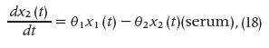
where x1 is the cortisol concentration in the adrenal glands and x2 is the serum cortisol concentration. θ1 and θ2, respectively, represent the infusion rate of cortisol from the adrenal glands into the blood and the clearance rate of cortisol by the liver. The equation

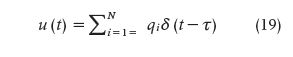
is an abstraction of the hormone pulses that result in cortisol secretion, where qi represents the amount of the hormone pulse initiated at time τi (qi is zero if a hormone pulse did not occur at time τi) and it was accepted that impulses occur at integer minute values. N corresponds to the length of the input (N = 1440). Blood was collected, beginning at y0 and, then, with a sampling interval of ten minutes, for M samples (M =144). The recovered pulses are mostly small at the beginning of the scheduled sleep, with a large pulse occurring toward the end of the sleep period or at the beginning of the wake period. Besides, there are also multiple small- and medium-sized pulses occurring during the wake period. r² values close to 1.0 suggest that the model is a good estimator.
Due to the simultaneous release and clearance of hormones and the unknown timing and amplitudes of the secretory events, identifying the pulsatile input to the system and the infusion and clearance rates is challenging. Moreover, due to data collection difficulties and cost, the sampling interval is usually relatively large (10–60 minutes) compared to the expected interpulse intervals as well as the secretion and clearance rates of cortisol. Hence, data resolution is low, making it difficult to identify delays and potential consecutive pulses. A third obstacle is cortisol secretion differences in sleep and wake states and at different circadian times. Finally, there is interindividual variation, even among healthy individuals. In summary, the proposed algorithm works well, even when pulses are not easily identifiable, and is still applicable to cases in which pulses can be identified by visual inspection.

The Future of Deconvolution Research

The concept of deconvolution is purely mathematical with a relatively recent incorporation in applied subjects and specifically in physiology, where the intestinal tract appears as its first exploratory area. This was followed more steadily for use in the field of renography but, surprisingly, also in endocrinology, with many contributions and rather sophisticated procedures. Based on this development, we dare anticipate further news, even though the method still faces instability difficulties that will no doubt call for researchers’ ingenuity. The simple matrix technique with its ill-conditioned characteristics poses an insurmountable drawback that needs to be dodged by a number of computational tricks, because a direct approach resembles trying to get through a thick, hard wall by sheer brute force. No way, but there is more than one way to skin a cat.
Questions about possible applications of the procedure in other physiological systems, other biological areas, or even in the environment come up readily, and the systems approach may lend us a hand in this respect.

References

1. A. A. Domínguez, “History of the convolution operation,” IEEE Pulse Mag., vol. 6, no. 1, pp. 38–49, Jan.–Feb. 2015.
2. N. Wiener, Extrapolation, Interpolation, and Smoothing of Stationary Time Series. Cambridge, MA: MIT Press, 1964.
3. L. Fejér, “Untersuchungen über Fouriersche Reihen (Investigations on the Fourier series),” Mathematische Annalen, vol. 58, pp. 51–69, 1903.
4. M. Riesz, “Über summierbare trigonometrische Reihen (On the summability of trigonometric series),” Mathematische Annalen, vol. 71, no. 1, pp. 54–75, 1911.
5. M. E. Valentinuzzi and E. M. Montaldo Volachec, “Discrete deconvolution,” Med. Biol. Eng., vol. 13, no. 1, pp. 123–125, Jan. 1975.
6. B. L. Diffey, F. M. Hall, and J. R. Corfield. “The 99mTc-DTPA dynamic renal scan with deconvolution analysis,” J. Nucl. Med., vol. 17, no. 5, pp. 352–355, May 1975.
7. A. González, D. Ros, and J. Pavia, “Estimate of relative function and transit time in renographic studies,” J. Nucl. Biol. Med., vol. 38, no. 3, pp. 502–507, Sept. 1994.
8. R. Lawson, “Quantitative methods in renography,” Sem. Nucl. Med., vol. 29, pp. 146–159, 1999.
9. L. A. Stevens, J. Coresh, T. Greene, and A. S. Levey, “Assessing kidney function: Measured and estimated glomerular filtration rate,” New Engl. J. Med., vol. 354, no. 23, pp. 2473–2483, June 2006.
10. S. R. Thomas, A. T. Layton, H. E. Layton, and L. C. Moore, “Kidney modeling: Status and perspectives,” Proc. IEEE, vol. 94, no. 4, 2006, pp. 740–752, Apr. 2006.
11. I. A. Al-Shakrah, “A comparison between the values of renal parenchymal mean transit time by applying two methods, matrix inversion deconvolution and Rutland- Patlak Plot,” World Appl. Sci., vol. 8, no. 10, pp. 1211–1219, 2010.
12. G. Segre, “Compartmental models in the analysis of intestinal absorption,” Protoplasma, vol. 63, no. 1–3, pp. 328–335, 1967.
13. J. D. Veldhuis, M. L. Carlson, and M. L. Johnson, “The pituitary gland secretes in bursts: Appraising the nature of glandular secretory impulses by simultaneous multiple- parameter deconvolution of plasma hormone concentrations,” Proc. Natl. Acad. Sci. USA, vol. 84, no. 21, pp. 7686–7690, Nov. 1987.
14. Johnson ML, Veldhuis JD, Eds., Quantitative Neuroendocrinology, vol. 28. New York: Academic Press, 1995.
15. M. H. Samuels, J. Veldhuis, C. Cawley, R. J. Urban, M. Luther, R. Bauer, and G. Mundy. (2013, July 10). Pulsatile secretion of parathyroid hormone in normal young subjects: Assessment by deconvolution analysis. J. Clin. Endocrinol. Metabol. [Online]. 77(2).
16. J. R. Kerrigan, J. D. Veldhuis, S. A. Leyo, A. Iranmanesh, and A. D. Rogol, “Estimation of daily cortisol production and clearance rates in normal pubertal males by deconvolution analysis,” J Clin. Endocrinol. Metab., vol. 76, no. 6, pp. 1505– 1510, June 1993. Online: July 1, 2013.
17. B. Tönshoff, J. D. Veldhuis, U. Heinrich, and O. Mehls, “Deconvolution analysis of spontaneous nocturnal growth hormone secretion in pre-pubertal children with pre-terminal chronic renal failure and with end-stage renal disease,” Pediatric Res., vol. 37, no. 1, pp. 86–93, Jan. 1995.
18. N. Hill, M. T. Dattani, E. Charmandari, D. R. Matthews, and P. C. (2011). Deconvolution analysis of 24-h serum cortisol profiles informs the amount and distribution of hydrocortisone replacement therapy. Endocrine Abstracts. [Online]. 27 OC1.5.
19. C. J. Peters, N. Hill, M. T. Dattani, E. Charmandari, D. R. Matthews, and P. C. Hindmarsh. (2013, Mar.). Deconvolution analysis of 24-h serum cortisol profiles informs the amount and distribution of hydrocortisone replacement therapy. Clin. Endocrinol. (Oxf.). [Online]. 78(3).
20. R. T. Faghih, M. A. Dahleh, G. K. Adler, E. B. Klerman, and E. N. Brown. (2014, Jan.). Deconvolution of serum cortisol levels by using compressed sensing. [Online]. 9(1). Available: http://www.plosone.org PLoS ONE/article/metrics/info:doi/10.1371/journal.pone.0085204#savedHeader.
21. E. N. Brown, P. M. Meehan, and A. P. Dempster, “A stochastic differential equation model of diurnal cortisol patterns,” Amer. J. Physiol.-Endocrinol. Metab., vol. 280, pp. E450–E461, Mar. 2001.
22. R. T. Faghih, K. Savla, M. A. Dahleh, and E. N. Brown, “A feedback control model for cortisol secretion,” Conf. Proc. IEEE Eng. Med. Biol Soc., Boston, MA, 2011, pp. 716–719. doi:10.1109/ IEMBS.2011.6090162.